Introduction: the lake whose river runs backwards
At the heart of Cambodia lies the largest lake in Southeast Asia: Tonle Sap Lake. In the dry season it is a calm body of water some 120 km long and 2,500 km² in area, but in the rainy season its surface area swells sevenfold, to about 17,500 km² (Siev et al., 2018).
Why does it transform so dramatically? The key is the 120-km-long Tonle Sap River, which connects the lake to the Mekong River. Twice a year, this river reverses the direction of its flow.
- Dry season (Nov–Apr): water from the lake drains down the river into the Mekong (normal flow).
- Rainy season (May–Oct): the swollen Mekong pushes water back up the river and into the lake (reverse flow).
This phenomenon — in which the river periodically reverses, like a beating heart, to refill the lake — is known as the flood pulse (Kummu & Sarkkula, 2008). It is one of the rarest hydrological phenomena on Earth, and it sustains Tonle Sap’s extraordinary fisheries and ecosystems.
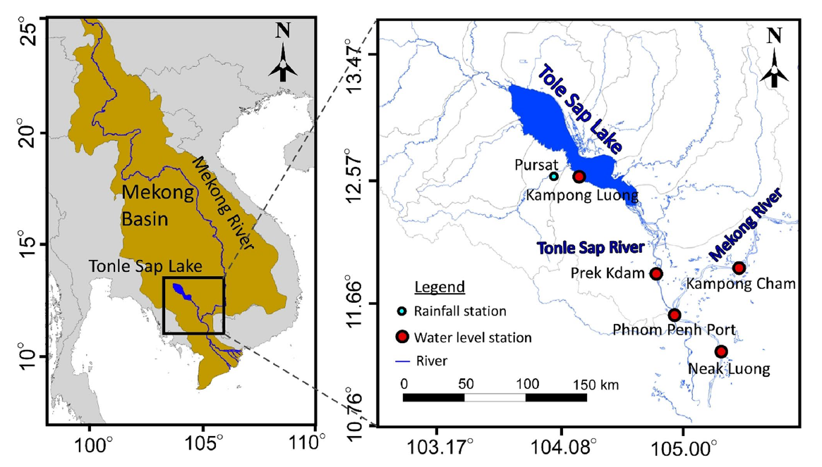
We analysed 15 years of daily water-level data (1998–2013) at five stations across this basin, quantifying how the flood pulse propagates from upstream to downstream and into the lake (Yang et al., 2017, 2022).
The central tool is the theme of this article: time-series analysis. Last time (#7) we used the FFT to extract the hidden periodicity in water levels. Here we go one step further and learn how to measure the “time lag” between two water-level signals. In other words, we answer — from data alone — the question:
Once the Mekong rises, how many days does it take for that signal to reach the lake?
“Seeing” the flood pulse — where the reversal appears
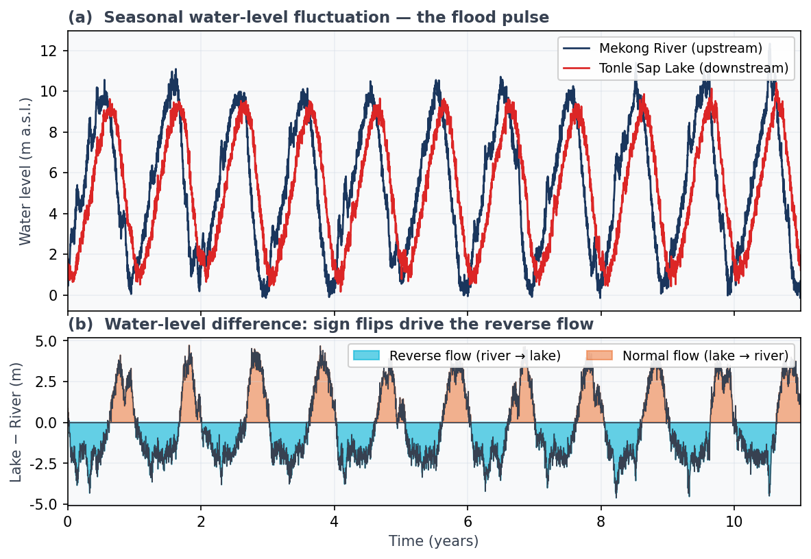
Let us first look at the phenomenon itself. Figure 2 shows the water levels of the upstream Mekong (navy) and the downstream Tonle Sap Lake (red).
Notice two things.
- Both signals oscillate with an ~1-year period (Figure 2 a) — the same seasonal periodicity we confirmed with the FFT last time.
- The lake’s peak lags slightly behind the river’s. The red curve seems to chase the navy one. This lag is precisely the time it takes for the flood pulse to travel from upstream to the lake.
Figure 2 (b) plots “lake level − river level.” When this difference is negative — when the river stands higher than the lake — water flows backwards, from river into lake (cyan region). The reverse flow is concentrated in roughly May–October, and its duration varies from 80 to 150 days from year to year (Yang et al., 2022).
So how do we extract this “lag” as an actual number, rather than by eye? We now introduce three tools, one at a time.
Tool 1: Auto-correlation — measuring a signal’s “memory”
The first tool is auto-correlation. It measures “how similar a time series is to a time-shifted copy of itself.”
The idea is simple. Take the water level \(x_t\), shift it by \(k\) days to obtain \(x_{t+k}\), and compute the correlation between the two. This is the auto-correlation coefficient at lag \(k\), \(r(k)\):
\[ r(k) = \frac{\sum_{t=1}^{n-k} (x_t - \bar{x})(x_{t+k} - \bar{x})}{\sum_{t=1}^{n}(x_t - \bar{x})^2} \]
(where \(\bar{x}\) is the mean and \(n\) the length). At \(k=0\) we compare the signal with itself, so \(r(0)=1\). As \(k\) grows:
- For a periodic signal, shifting by one full period brings the shape back into alignment, so \(r(k)\) oscillates and peaks at integer multiples of the period.
- For a non-periodic signal (e.g. random noise), even a small shift destroys the resemblance, so \(r(k)\) drops quickly to zero.
Figure 3 shows the auto-correlation of water level (periodic) and rainfall (non-periodic).
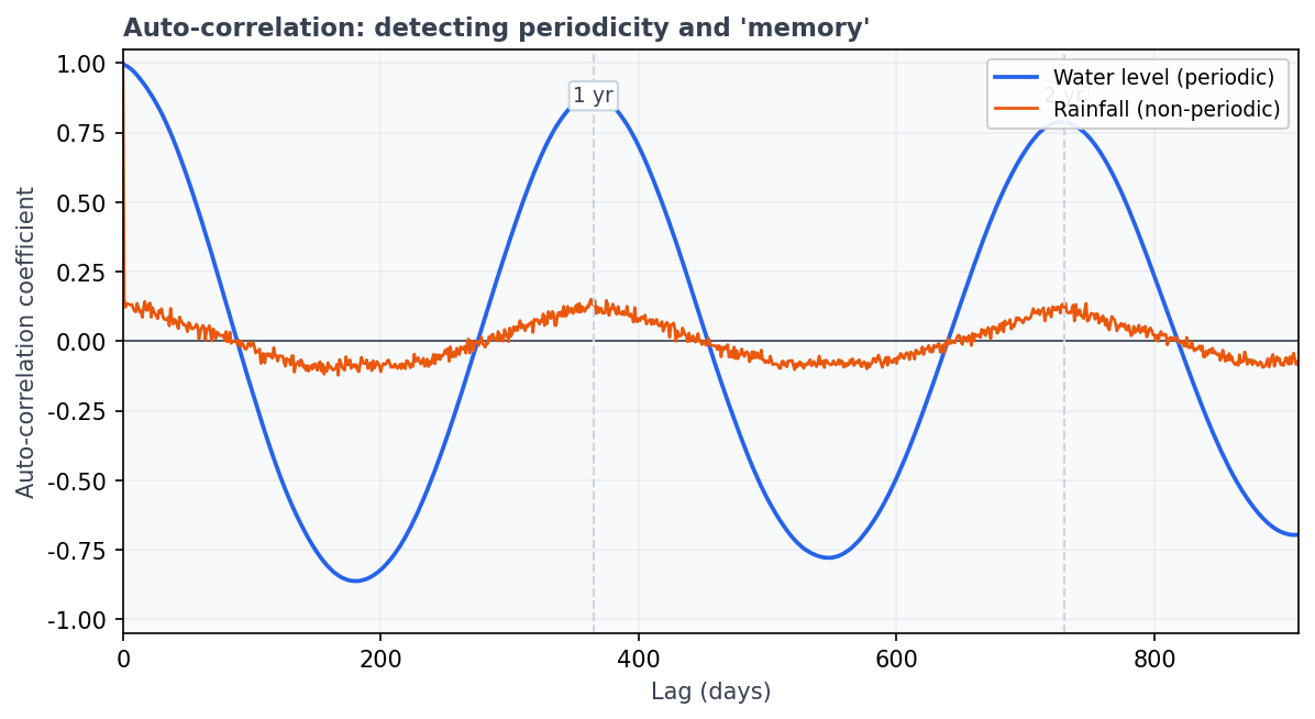
Water level (blue) peaks cleanly at a lag of 365 days. This is direct evidence that the water level “resembles its own state one year earlier” — that is, it has a 1-year period. That the peaks decay only slowly means the system has long memory: past states leave a long tail.
Rainfall (orange), by contrast, sinks to near zero almost immediately. Rain is a short-memory process — “it rained yesterday” tells you little about today. Auto-correlation diagnoses this presence or absence of periodicity and memory at a glance.
Takeaway: Auto-correlation measures how strongly a single time series is linked to its own past. It is the starting point for judging whether a periodicity exists and whether memory is long or short.
Tool 2: Cross-correlation — measuring the time lag between two signals
Where auto-correlation works on a single series, cross-correlation compares two different series. The idea is almost the same: shift one series \(x_t\) (say, the upstream river) by \(k\) and measure its correlation with the other, \(y_t\) (the lake):
\[ r_{xy}(k) = \frac{1}{n}\sum_{t=1}^{n-k}\frac{(x_t - \bar{x})(y_{t+k}-\bar{y})}{\sigma_x \sigma_y} \]
where \(\sigma_x, \sigma_y\) are the standard deviations. We sweep \(k\) from negative to positive, compute \(r_{xy}(k)\), and find the lag \(k\) that maximises the cross-correlation. That \(k\) is the time lag between the two series (Larocque et al., 1998).
Figure 4 gives a worked example.
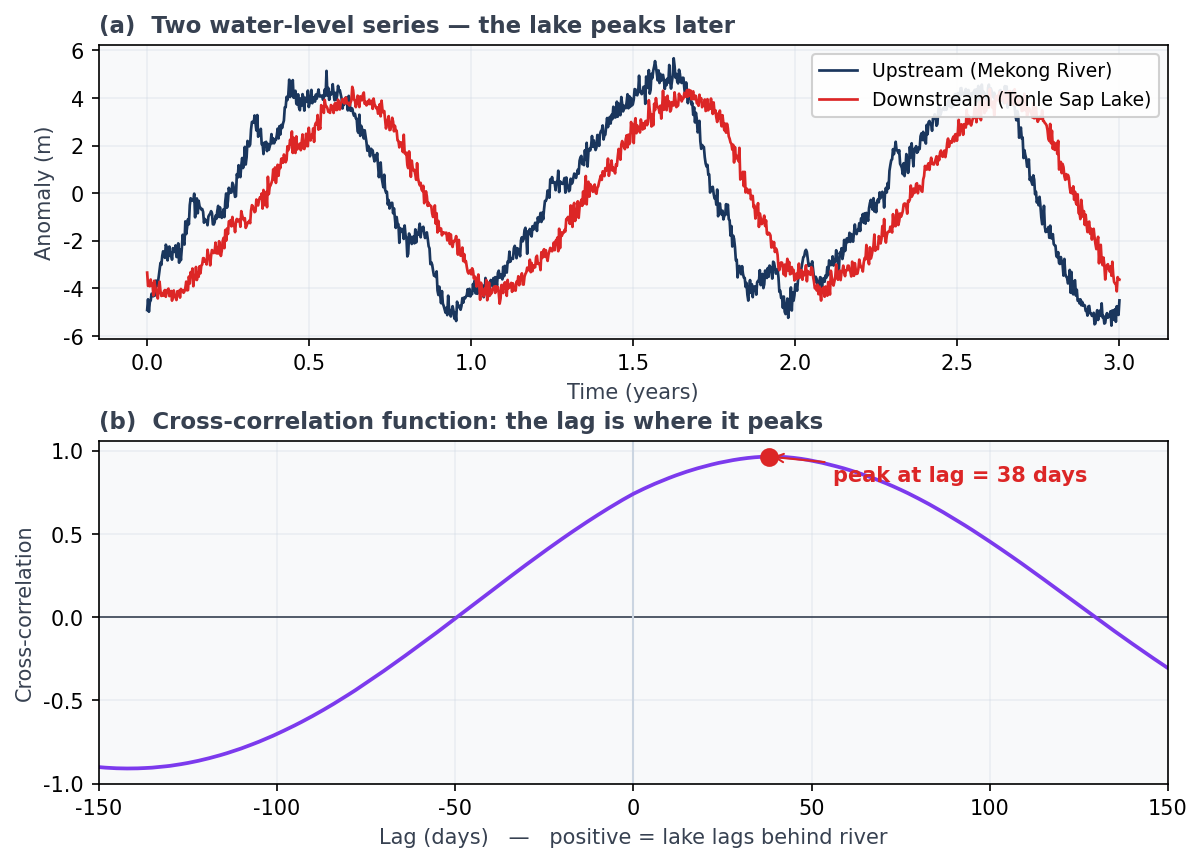
The cross-correlation function (Figure 4 b) peaks at a lag of about 38 days, meaning the Mekong’s water-level variation takes roughly 38 days to reach Tonle Sap Lake. In the actual study, the lake (KL) lagged the mid-river station PK by 37 ± 7 days and the junction PPP by 49 ± 7 days (Yang et al., 2017). Dividing by river distance, the flood pulse’s propagation speed was estimated at about 3.5 km/day.
Cross-correlating rainfall with the lake level gives another result: “the lake responds to rain about 80 days later” (Yang et al., 2017). An invisible “time lag” thus emerges as a concrete number of days.
The computation takes only a few lines of Python. To illustrate the idea (run it on your own data):
import numpy as np

def cross_correlation(x, y, maxlag):
    """Shift y relative to x and compute the cross-correlation."""
    x = (x - x.mean()) / x.std()
    y = (y - y.mean()) / y.std()
    n = len(x)
    full = np.correlate(y, x, mode="full") / n      # all lags
    mid = n - 1
    lags = np.arange(-maxlag, maxlag + 1)
    vals = full[mid - maxlag: mid + maxlag + 1]
    return lags, vals

lags, vals = cross_correlation(river_level, lake_level, maxlag=150)
time_lag = lags[np.argmax(vals)]                    # lag of the peak = time lag
print(f"Estimated time lag: {time_lag} days")
Takeaway: Cross-correlation measures how — and with what delay — two time series resemble each other. The location of the peak is the time lag, from which even the speed of propagation can be quantified.
Tool 3: Cross-wavelet — tracking a lag that changes over time
Cross-correlation has one weakness: it yields only a single lag, averaged over the whole record. But nature changes its relationships from year to year and season to season. In years of dam construction or extreme weather, the way the signal propagates can itself change.
Enter the cross-wavelet transform (XWT), the natural successor to the FFT. Whereas the FFT collapses an entire series into one frequency spectrum, the wavelet transform spreads it out over a time–period plane, telling us when, at which period, and how strong each fluctuation was (Torrence & Compo, 1998).
Taking the wavelet transforms \(W^X, W^Y\) of the two series, their product
\[ W^{XY} = W^X \, \overline{W^Y} \]
(where the overbar denotes complex conjugation) is the cross-wavelet. The phase angle \(\arg(W^{XY})\) of this complex number gives the phase difference between the two series at each time and period. That phase difference can be converted into how many days the wave at that period is shifted — i.e. the time lag (Grinsted et al., 2004).
Figure 5 shows the result.
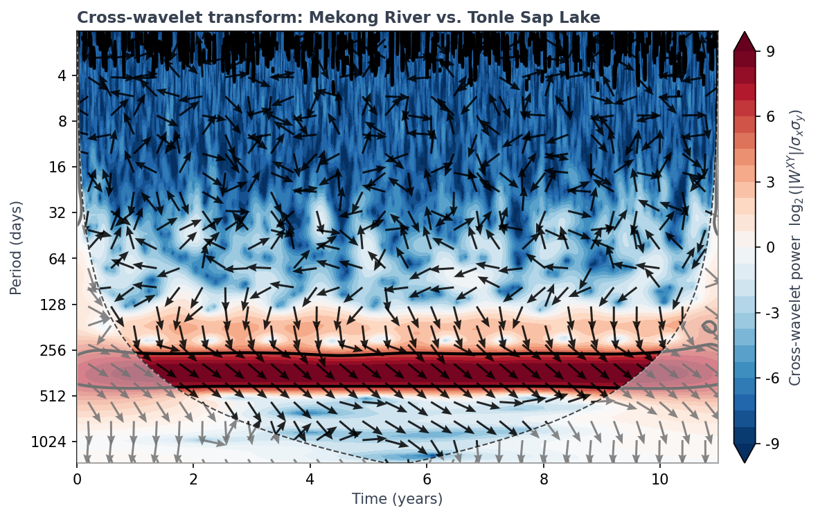
How to read this plot — colour and arrows separately
A cross-wavelet plot carries two pieces of information at once: colour (power) and arrows (phase). The trick, for beginners, is to read them one at a time.
① Colour = power (how strongly the two signals oscillate at the same period, at the same time)
- The redder it is, the more both signals oscillate together and strongly at that time and period (the shared variation is strong). Bluer means weaker.
- Inside the thick black contour, the signal is statistically significant (the 5% level — unlikely to be chance).
- Outside the dashed line (the COI) the edges are unreliable, so don’t read it.
In Figure 5, the 256–512-day (~1-year) band is bright red, so we read “river and lake are strongly coupled at a 1-year period.”
② Arrows = phase (the direction of the “time shift” between the two signals)
The arrow direction shows how the two signals are shifted relative to each other (Figure 6).
- → pointing right: in-phase. The two move in step (lag ≈ 0).
- ← pointing left: anti-phase. When one is at a peak, the other is at a trough (shifted by half a period).
- ↓ pointing down: the river (series 1) leads the lake (series 2) by ¼ period.
- ↑ pointing up: the reverse (the lake leads the river).
- A slanted arrow: in between; the tilt angle θ is exactly “how big the shift is.”
So in Figure 5, the arrows in the annual band point down-right, meaning “almost in-phase (right) but with the river leading slightly (down)” — i.e. the river moves just a little earlier.
The cross-wavelet phase is “(phase of series 1) − (phase of series 2).” So which of the two you pass as the first argument flips the sign of the phase and the up/down tilt of the arrows (the physics is unchanged).
| Ordering | Phase | Arrow | Example |
|---|---|---|---|
xwt(river, lake) (the leading river first) |
+39.7° | down-right | Figure 5 in this article |
xwt(lake, river) (the lagging lake first) |
−35.9° | up-right | Yang et al. (2017) |
Both express the same fact — “the river leads the lake by about 40 days.” The 2017 paper put the lake (KL) first (xwt(KL, PK)), which is why its phase is negative; the sign is merely a matter of ordering. The hand calculation below uses the magnitude \(35.9°\), to match the paper.
The high-power band stretching horizontally across the annual period (256–512 days) tells us the flood pulse’s annual cycle dominated for all 15 years. And because the arrows (phase) point consistently down and to the right, we read that river and lake moved together while maintaining a stable phase difference — a steady time lag. Had the arrows scrambled partway through, that would have signalled “the propagation changed in some particular year.” The cross-wavelet thus reveals the time variation of the lag that cross-correlation cannot see.
Moreover, the phase angle \(\theta\) in the significant band converts directly into a time lag. With wavelength (period) \(T\),
\[ \text{time lag} = \frac{\theta}{2\pi} \, T \]
In the actual study, the mean phase of \(-35.9°\) in the 374-day band yielded a lag of 37.3 days (KL–PK), consistent with the cross-correlation result (Yang et al., 2017). For the synthetic data of Figure 5 too, a phase of about 40° converts to a lag of roughly 41 days, agreeing well with the cross-correlation (~38 days). Two independent methods arriving at the same answer is what lends the result its credibility.
You can do this with pen and paper. Take the paper’s KL–PK case (374-day band).
- Read the phase angle off the plot: \(\theta = 35.9°\) (the river leads the lake).
- Ask “what fraction of one full cycle (360°) is this shift?”: \(35.9 \div 360 = 0.0997\) (about one tenth).
- Multiply that fraction by the period \(T = 374\) days: \(0.0997 \times 374 \approx \mathbf{37\ \text{days}}\).
→ We read it as “the lake’s annual peak arrives about 37 days after the river’s.”
Using radians gives the same result: \(\text{time lag} = \dfrac{\theta_{\text{rad}}}{2\pi}\,T = \dfrac{0.6266}{6.283}\times 374 \approx 37\ \text{days}\) — and it agrees with the ~40 days from cross-correlation.
The cross-wavelet figure in this article was drawn with a dependency-free Python port of the MATLAB Grinsted toolbox (Grinsted et al., 2004) used in the original paper. Usage is roughly as follows — just pass two time series and the sampling interval.
from xwt_grinsted import xwt, plot_xwt, phase_to_timelag

# x, y : two water-level series (uniform spacing, same dt), dt = 1.0 (day)
Wxy, period, scale, coi, sig95, t, sigmas = xwt(x, y, dt=1.0)

# Plot in the 2017-paper style (significance contour, COI, phase arrows)
plot_xwt(t, period, Wxy, coi, sig95, dt=1.0, sigmas=sigmas, out="xwt.png")

# Convert phase to time lag in the 374-day band: timelag = θ·T / 2π
lag, theta, P = phase_to_timelag(Wxy, period, target_period=374)
print(f"Time lag: {lag:.1f} days (mean phase {np.degrees(theta):.1f} deg, period {P:.0f} d)")
Tying it together — the division of labour among the three tools
Through the Tonle Sap analysis we have met three tools of time-series analysis. Let us summarise their roles.
| Tool | What it measures | Answer for Tonle Sap |
|---|---|---|
| Auto-correlation | Periodicity and memory of one series | Water level has a 1-year cycle and long memory |
| Cross-correlation | Average time lag between two series | River→lake ≈ 40 days; rain→lake ≈ 80 days |
| Cross-wavelet | Time-varying phase and lag | The 1-year cycle dominated consistently for 15 years |
Notice how we widened our view one step at a time: “one series → two series → variation in time.” This three-stage structure is a general template, applicable not only to Tonle Sap but to any hydrological time series.
Indeed, these results later fed a lag-based multiple-regression model that predicts and interpolates downstream and lake water levels from the upstream level, reproducing observations with both \(R^2\) and NSE exceeding 0.99 (Yang et al., 2022). Measuring the “time lag” correctly leads directly to the practical tasks of filling data gaps and forecasting.
To groundwater — the same tools work beneath the ground
So far we have discussed surface water (river and lake). But this is a series on groundwater science. Why tell this story? The answer is simple: exactly the same tools work beneath the ground.
Groundwater level, too, is a time series that responds — with a delay — to an external “input.” For example:
- Ocean tide → coastal groundwater level: each time the sea rises and falls, its pressure propagates through the aquifer inland and rocks the water table. At Minami-Daito Island in #7, the tide made the freshwater lens “breathe” (Yang et al., 2020). Cross-correlating sea level with each monitoring well yields “the time lag for the tidal peak to reach the well,” from which the aquifer’s permeability can be estimated.
- Atmospheric pressure → unconfined groundwater level: when air pressure falls, the water table rises slightly. This barometric response is observed in the unconfined groundwater of Beppu, too. The cross-correlation of pressure and level becomes a mirror of the geology.
Chasing a lake’s level with a river’s level, or a well’s level with the ocean tide, is mathematically the same problem: “measuring the time lag between two time series.” The tools learned at Tonle Sap carry over directly to groundwater analysis. That is why a distant Cambodian lake belongs in an introduction to groundwater science.
Summary
- In Tonle Sap Lake, the rainy-season Mekong reverses up the river to fill the lake — the flood pulse. We quantified its propagation with time-series analysis.
- Auto-correlation measures the periodicity and memory of one series. The water level proved to have a 1-year cycle and long memory.
- Cross-correlation measures the time lag between two series. The Mekong’s variation reaches the lake in ~40 days; rain’s influence appears ~80 days later.
- Cross-wavelet reveals a phase/lag that varies in time. The flood pulse’s annual cycle dominated consistently for 15 years.
- These tools transfer directly to the response of groundwater level to ocean tides and air pressure, leading to estimates of aquifer permeability.
We have seen that cross-correlation can measure a “time lag.” But why does the response delay differ from well to well for the same input? Next time we step into the equation of pressure propagation and uncover how the geology’s permeability (hydraulic diffusivity) and depth determine the lag.
References
- Yang, H., Siev, S., Yoshimura, C., Fujii, H. (2017) Identification of phase propagation of water level between the Tonle Sap Lake and River based on time series analysis. Proceedings of the 2nd International Symposium on Conservation and Management of Tropical Lakes, 16–22.
- Yang, H., Siev, S., Uk, S., Yoshimura, C. (2022) Relationship between water levels and flood pulse induced by river–lake interaction in the Tonle Sap basin, Cambodia. Environmental Earth Sciences, 81, 226. https://doi.org/10.1007/s12665-022-10353-5
- Yang, H., Shimada, J., Okumura, A., Shibata, T., Pinti, D.L. (2020) Freshwater lens oscillation induced by sea tides and variable rainfall at the uplifted atoll island of Minami-Daito, Japan. Hydrogeology Journal, 28, 2105–2114. https://doi.org/10.1007/s10040-020-02185-z
- Kummu, M., Sarkkula, J. (2008) Impact of the Mekong River flow alteration on the Tonle Sap flood pulse. Ambio, 37, 185–192.
- Siev, S., Yang, H., Sok, T., Uk, S., Song, L., Kodikara, D., Oeurng, C., Hul, S., Yoshimura, C. (2018) Sediment dynamics in a large shallow lake characterized by seasonal flood pulse in Southeast Asia. Science of the Total Environment, 631–632, 597–607.
- Torrence, C., Compo, G.P. (1998) A practical guide to wavelet analysis. Bulletin of the American Meteorological Society, 79, 61–78.
- Grinsted, A., Moore, J.C., Jevrejeva, S. (2004) Application of the cross wavelet transform and wavelet coherence to geophysical time series. Nonlinear Processes in Geophysics, 11, 561–566.
- Larocque, M., Mangin, A., Razack, M., Banton, O. (1998) Contribution of correlation and spectral analyses to the regional study of a large karst aquifer (Charente, France). Journal of Hydrology, 205, 217–231.