A well is already recording the movement of the Earth
On 26 September 2003, a magnitude 8.0 earthquake struck off Tokachi, Hokkaido. In observation wells across the island the groundwater level jumped in a step at the moment of the earthquake. Some wells fell by tens of millimetres; others rose. When the shaking stopped, the levels did not return to where they had been.
The wells did not shake. The crust itself deformed, and that deformation was transmitted to the pore pressure of the aquifer. The well acted not as a seismometer but as a strain meter.
This article is about reading the dynamics of the Earth — earthquakes and eruptions — from a single time series of groundwater level. There are three stages: nineteen wells in Hokkaido, the 2000 eruption of Usu volcano, and the 1989 Loma Prieta earthquake.
Three faces of a well
Groundwater does not respond to an earthquake in one way. It shows three faces on three different time scales (Figure 1).
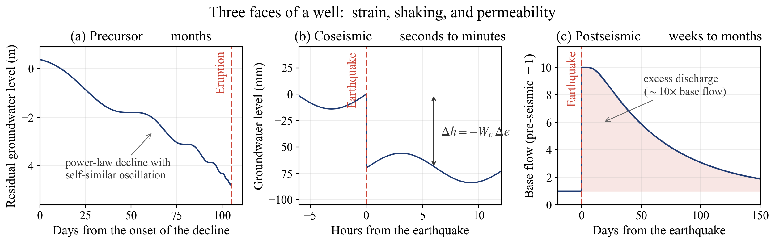
The precursor (months) is the faint signal of rock approaching failure. The coseismic response (seconds to minutes) is an elastic reaction to the static volumetric strain that fault slip imposes on the surrounding crust. The postseismic change (weeks to months) is irreversible: shaking opens fractures and alters the permeability of the crust itself.
Three quite different physics. Yet all three appear in the same record of water level. This article takes them in turn, with the technical heart in the second one — poroelasticity.
Recap: a well responds to whatever pushes on it
Before the main subject, it is worth restating the view this series has been building.
In #6 we saw the unconfined groundwater level at Beppu respond to barometric pressure: when the air presses harder on the aquifer, the level falls. In #9 we saw the level on Minami-Daito Island respond to ocean tides, and used the phase lag to estimate hydraulic conductivity across the island.
What these share is a view of the well as a device that records the forces applied to it from outside. Barometric pressure is a load from above; the tide is the load of seawater plus the deformation of the solid Earth. If that is so, the strain an earthquake imposes on the crust should be recordable by the same well.
This article extends that view to crustal strain. The tools are the same as well: the harmonic analysis used in #9 to isolate tidal constituents is exactly what calibrates the strain meter here.
Coseismic — measuring strain with a water level
First, get hold of “volumetric strain”
The protagonist of this section is volumetric strain \(\Delta\varepsilon\). The name sounds forbidding; the content is simple. It is just the fraction by which a volume has changed.
\[\Delta\varepsilon = \frac{\Delta V}{V}\]
A volume divided by a volume, so it carries no units. Stretched and expanded, it is positive; squeezed and shrunk, negative.
A sense of scale helps. The strains at issue in seismology are of order \(10^{-8}\) to \(10^{-6}\). A strain of \(10^{-8}\) means a block of rock 1 km long stretching by 0.01 mm — invisible to the eye and to surveying. Yet that deformation moves the level in a well by several millimetres. This is why a well makes such a good strain meter.
Why does a change in volume appear as a change in level? The left half of Figure 2 is the whole story.
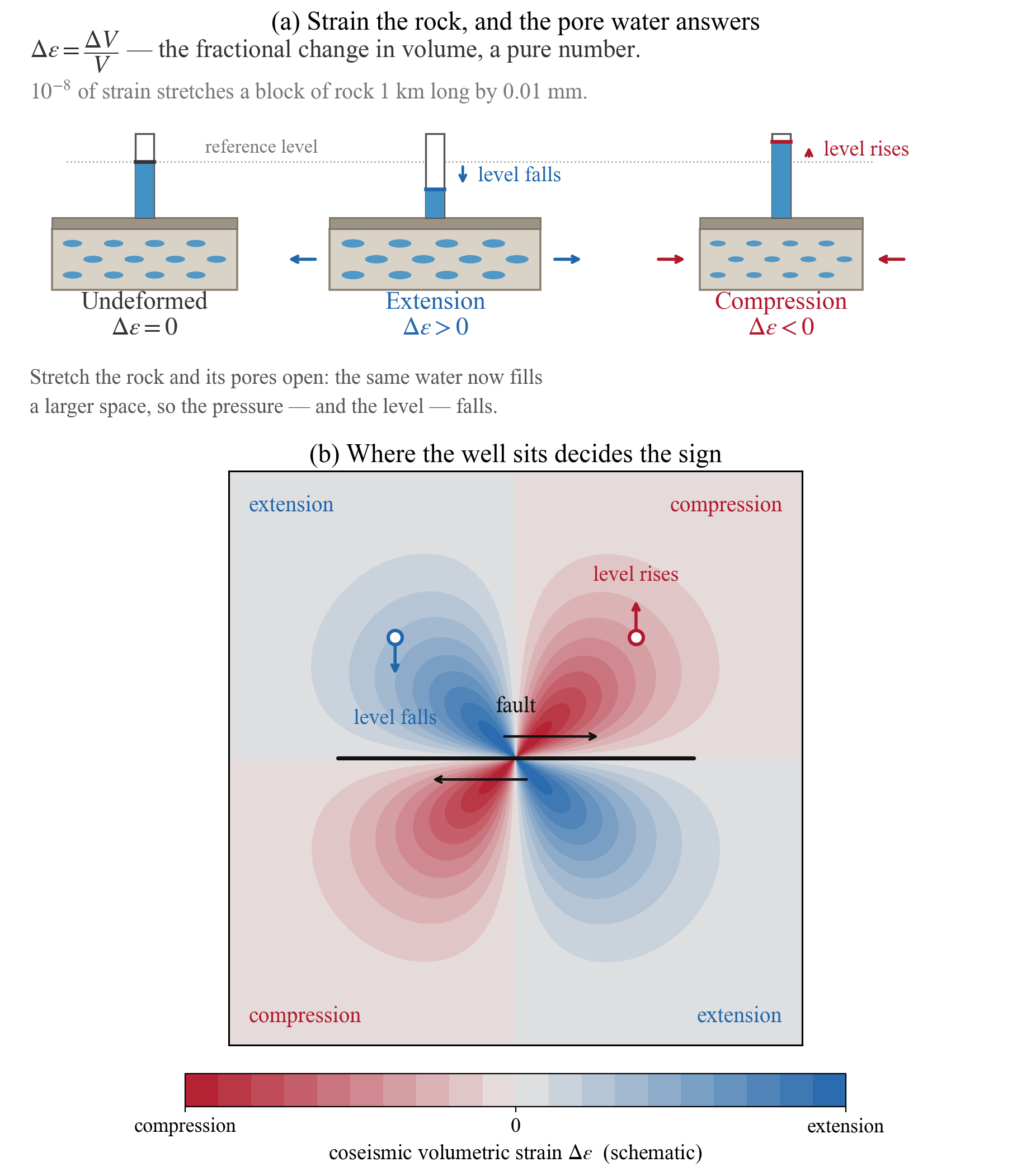
The point fits in one line. Stretch the rock framework and the pores open. Put the same water in a larger space and the pressure falls. The level in a standpipe is only that pressure rendered as a height.
And as the right half of Figure 2 shows, extension and compression are laid out in quadrants around a fault. In one and the same earthquake, the level falls at some wells and rises at others, depending on where they stand.
Putting it in an equation
In a confined aquifer, the change in groundwater level \(\Delta h\) and the change in volumetric strain \(\Delta\varepsilon\) are linearly related:
\[\Delta h = -\frac{B K_u}{\rho_w g}\,\Delta\varepsilon = -W_{\varepsilon}\,\Delta\varepsilon\]
The symbols are as follows (Jacob, 1940; Wang, 2000).
| Symbol | Name | Meaning and units |
|---|---|---|
| \(\Delta h\) | Change in groundwater level | What is observed. m or mm |
| \(\Delta\varepsilon\) | Change in volumetric strain | What is wanted. \(\Delta V/V\), dimensionless |
| \(W_{\varepsilon}\) | Strain sensitivity | Metres of level per unit strain. m. The per-well calibration |
| \(B\) | Skempton’s coefficient | The share of an applied stress carried by the pore fluid. 0–1, dimensionless |
| \(K_u\) | Undrained bulk modulus | Stiffness of the rock when the water cannot escape. Pa (usually quoted in GPa) |
| \(\rho_w\) | Density of water | About 1000 kg m⁻³ |
| \(g\) | Gravitational acceleration | About 9.8 m s⁻² |
\(B\) and \(K_u\) are properties of the rock; \(\rho_w g\) converts a pressure into a height of water. Knowing the single lumped coefficient \(W_{\varepsilon}\) is enough to read strain from level.
The minus sign is essential. When the volumetric strain is positive (extension), the level falls — exactly as in Figure 2.
\(W_{\varepsilon}\) differs from aquifer to aquifer. Given the same strain, a stiff rock aquifer and a soft sedimentary one produce different steps. Knowing \(W_{\varepsilon}\) is therefore exactly what it means to calibrate a well as a strain meter.
The Moon does the calibration for you
How is \(W_{\varepsilon}\) determined? This is where the tide earns its keep.
The Moon and the Sun deform the crust every day, reliably. The theoretical volumetric strain can be computed from solid-earth tides plus ocean tide loading (Shibata et al. 2010 used GOTIC2). From the observed record, one extracts the component at the same period. The M₂ constituent (period 12.4206 h) has the largest tidal strain amplitude, and its period exceeds 12 h, which keeps it away from the diurnal peaks of temperature and barometric effects — that is why M₂ is chosen.
\[W_{\varepsilon}^{(M_2)} = \frac{T_W}{T_T}\]
where \(T_W\) is the M₂ amplitude of the water level and \(T_T\) that of the theoretical volumetric strain. The amplitude and phase on the water-level side are extracted with the Bayesian tidal analysis program BAYTAP-G.
Figure 3 shows the whole calibration.
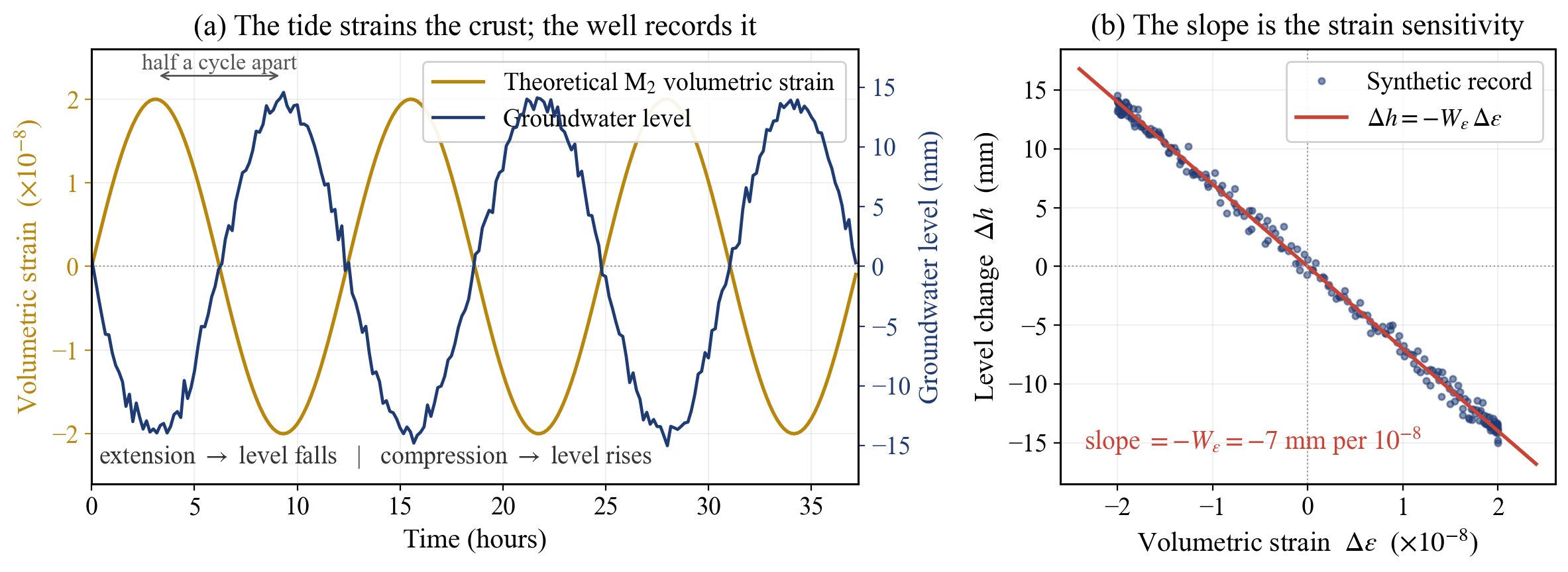
In the left panel the two curves move as mirror images. That anti-phase is the minus sign made visible. In the right panel the same record folds onto a single line whose slope is \(-W_{\varepsilon}\).
When an earthquake arrives, the line jumps
Once calibrated, the well simply has to be read. Fault slip imposes a static step of volumetric strain on the surrounding crust, with extension and compression distributed in the familiar four-quadrant pattern about the fault.
\[\Delta h_{\text{eq}} = -W_{\varepsilon}^{(E)}\,\Delta\varepsilon_{\text{eq}}\]
Figure 4 places a well in an extensional zone beside one in a compressional zone, for the same magnitude of strain step.
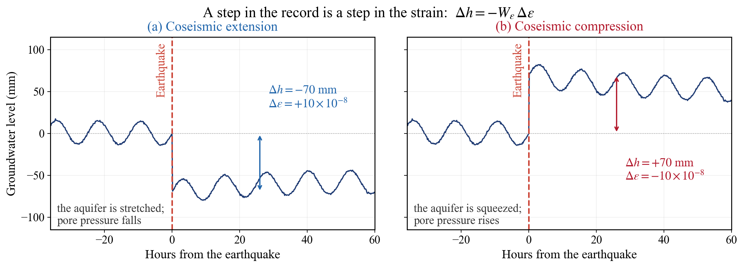
The sign of the step tells you the sign of the strain at that place; the amplitude tells you its size. The well works as a strain meter drilled into the ground.
Do the two answers agree?
Here lies the core of Shibata et al. (2010). For nineteen wells in Hokkaido they estimated \(W_{\varepsilon}\) by two independent routes and compared them.
One is the tidal route, \(W_{\varepsilon}^{(M_2)}\), described above. The other is \(W_{\varepsilon}^{(E)}\), obtained from the coseismic steps produced by six earthquakes of magnitude 7 or greater between 1993 and 2004: the 1993 Kushiro-oki (M7.6), the 1993 Hokkaido-Nansei-oki (M7.8), the 1994 Hokkaido-Toho-oki (M8.1), the 1994 Sanriku-Haruka-oki (M7.5), the 2003 Tokachi-oki (M8.0) and the 2004 Kushiro-oki (M7.1). The theoretical coseismic strain was computed with Okada’s (1992) code.
The two estimates showed a good linear correlation. That two entirely different forcings — the tide of the Moon and the rupture of a fault — yield the same coefficient means the response of the groundwater level is governed by one framework: linear poroelasticity.
They also obtained the loading efficiency \(\gamma\) from the barometric response — the very quantity treated in #6, a dimensionless number giving the fraction of an increase in atmospheric pressure that is taken up by the pore pressure. They found \(\gamma = 0.16\)–\(0.62\) across the nineteen wells. Combining \(\gamma\) with \(W_{\varepsilon}\) yields the uniaxial undrained bulk modulus \(K_v^{(u)}\) of the aquifer. The values obtained correspond roughly to laboratory measurements for sandstone (13–47 GPa) and granite (61–66 GPa) (Wang, 2000).
In other words — from a single time series of water level, one can read the stiffness of the rock below.
Some wells do not cooperate
Not all nineteen wells were well behaved. At eight of them (AB, NW, OB6, SK, SR2, TS, YC, YN) the phase of the tidal response departed from the theoretical strain.
All but OB6 and TS lie within 2 km of the coast. At those wells the ocean tide loading contributed more than 80% of the M₂ tidal volumetric strain attributable to the solid earth tide. Either the theoretical ocean loading is itself inaccurate there, or something absent from the equation — such as direct flow of seawater into the aquifer — is at work.
The paper states the mismatch plainly. Linear poroelasticity does not explain every observation. That honesty leads directly to the next section.
Precursor — the groundwater moves before the eruption
Usu volcano, 2000
At 13:07 on 31 March 2000, Usu volcano in Hokkaido erupted. For three months beforehand, something strange had been happening in observation well GSH-1, 1200 m deep and within 2 km of the northern flank.
The well taps a confined fractured-rock aquifer in silicified rock, so its level tracks the pore pressure faithfully. After removing barometric and earth-tide effects with BAYTAP-G, the residual record separates into three periods (Shibata, Matsumoto & Akita, 2003):
- P1 (until 06:00 on 14 December 1999): steady variation
- P2 (14 December 06:00 – 28 March 2000 00:00): a power-law decline accompanied by self-similar oscillation
- P3 (from 28 March 00:00): irregular drawdown
Microearthquakes and crustal deformation began abruptly beneath the volcano around 20:00 on 27 March, and a larger earthquake was recorded at 00:23 on 28 March. The end of P2 coincides with the moment the rock began to fail in earnest.
The decline through P2 amounted to about 5 m. Read through the strain sensitivity obtained from the tidal response (7 mm per \(10^{-8}\) strain), this corresponds to more than \(7\times10^{-6}\) of tensional strain. Rising magma had been quietly stretching the surrounding rock.
The peculiar rhythm of a system approaching failure
This is where it becomes interesting. The authors fitted a log-periodic oscillation to the water level:
\[f(t) = A + B\,(t_c - t)^{m}\left\{1 + C\cos\left[\omega\ln(t_c - t) + \psi\right]\right\}\]
Here \(f(t)\) is the residual water level at time \(t\) and \(t_c\) is the critical failure point — the moment the rock breaks. The exponent \(m\) sets how fast the approach to failure accelerates; \(\omega\) sets how tightly the oscillation is spaced. \(A\), \(B\), \(C\) and \(\psi\) are fitted constants: \(A\) the final level, \(B\) the total drawdown, \(C\) the amplitude of the oscillation, \(\psi\) its phase.
Read as words: the first part, \((t_c-t)^m\), is the backbone that descends smoothly towards the failure point. The second part, \(\cos[\omega\ln(t_c-t)+\psi]\), is the wobble about that backbone. The logarithm is the essential ingredient: the oscillation repeats at equal intervals in logarithmic time, which means faster and faster in real time. It arises naturally when interactions among microcracks develop a hierarchy of scales.
Figure 5 is a reconstruction.
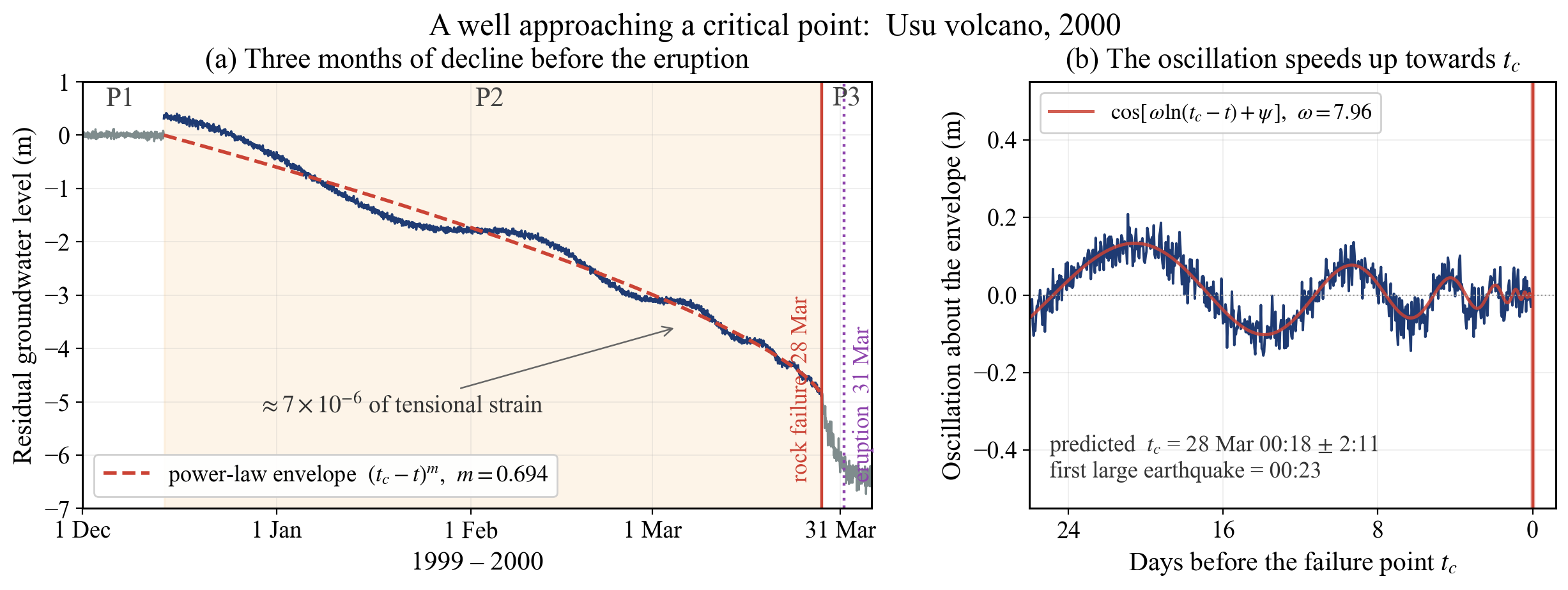
The fit gave critical exponents \(m = 0.694 \pm 0.006\) and \(\omega = 7.96 \pm 0.05\), with \(\omega\) inside the range (6–12) found in earlier studies. The power spectra in P2 and P3 follow a power law with exponent 1.77, giving a fractal dimension \(D = 2.62\) — close to the 2.25–2.75 obtained from acoustic emission experiments on fracturing rock.
And the striking result: the predicted failure point \(t_c\) was 00:18 ± 2:11 on 28 March, while the first large earthquake actually occurred at 00:23.
But this is not prediction
The result is seductive. It is worth stopping here.
As the paper itself reports honestly, re-estimating \(t_c\) as the data window lengthened did not give a stable answer. Until 30 January, \(m\) and \(\omega\) settled and \(t_c\) converged near 23 March. From about 20 February, however, \(t_c\), \(m\) and \(\omega\) all began to increase, peaked in early March, and returned to their February values between mid and late March. The authors attribute this to real changes in crustal strain and microcrack accumulation rather than to any artefact of the fitting.
In hindsight the agreement is remarkable. But there is no way, while living through it, to know whether today is 20 February or 20 March. Groundwater precursors remain a field where reproducibility and specificity — can we say nothing else would produce this? — are still debated. This article does not present the result as evidence that eruptions can be predicted. Rock approaching failure sometimes shows a characteristic rhythm through the window of a water level — that is as far as the evidence goes.
Postseismic — the earthquake changes the permeability of the crust
Loma Prieta, 1989
On 17 October 1989 the Loma Prieta earthquake struck California. Three changes were observed around the epicentre (Rojstaczer, Wolf & Michel, 1995):
- Stream flow increased rapidly — generally within 15 minutes of the earthquake
- The ionic concentration of stream water rose — while the ionic composition stayed essentially constant
- The water table dropped — over weeks to months after the earthquake
Increased spring and stream flow after a large earthquake had long been known. Two mechanisms competed to explain it.
Hypothesis A: elastic compression. The earthquake compresses the upper to middle crust and squeezes water upward. If true, sampling post-seismic springs means sampling fluids from depth.
Hypothesis B: shallow permeability enhancement. Strong shaking opens fractures in the shallow crust and water flows more easily. If true, what one observes says only something about shallow rheology.
The implications differ completely.
The decisive fact is that the water table fell
The observation Rojstaczer and colleagues found decisive was the third.
The water table dropped even at locations more than 15 km from the rupture zone — in the same region where stream flow increased. Elastic compression cannot account for this. If compression were forcing water up from depth, the water table should rise, not fall.
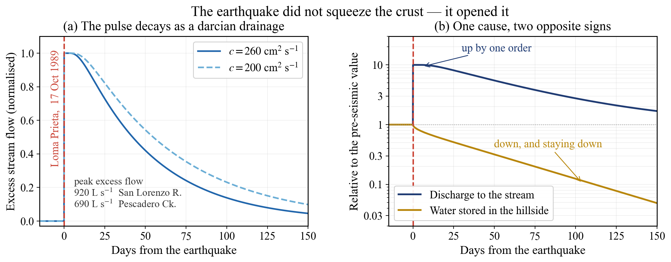
Permeability enhancement explains both at once. Open the fractures and groundwater drains to the streams faster. Recharge, however, does not increase. Storage therefore falls and the water table drops. More water leaving for the stream and less water remaining below are two faces of one cause (Figure 6).
Checking it with numbers
The argument does not stop at the qualitative. Base flow increased by about an order of magnitude within days, implying that basin-average permeability increased on average by an order of magnitude. Achieving that requires the open fracture apertures controlling permeability to widen by tens to hundreds of micrometres. Pre-earthquake basin-average permeability was estimated at about 10 millidarcies, and an aperture change of this size is unremarkable for the weak shallow crust of the region.
They then reproduced the decay of the excess flow with a simple darcian diffusion model. Solving the drainage of an initially triangular water table beneath a hillside gives the flux into the stream as
\[v = \frac{4k\rho g w}{\eta L}\sum_{n=0}^{\infty}\frac{(-1)^n}{2n+1}\exp\left[-\frac{(2n+1)^2\pi^2 c\,t}{4L^2}\right]\]
Here \(v\) is the groundwater flux into the stream, \(k\) the permeability, \(\rho\) the density and \(\eta\) the viscosity of water, \(w\) the maximum height of the water table above the stream, \(L\) the maximum length of the flow path, and \(c\) the hydraulic diffusivity — the rate at which a pressure change spreads through the ground. The infinite sum over \(n\) superposes the ways a hillside can drain; the higher terms die away fastest, so after a while only the first term survives and the decay becomes a simple exponential.
Observations at the San Lorenzo River (peak excess flow 920 L s⁻¹) and Pescadero Creek (690 L s⁻¹) were matched with \(c = 260\) and \(200\) cm² s⁻¹ respectively. The total excess flow generated by the earthquake reached \(1.1\times10^{7}\) m³, about 65% of it from these two catchments.
The earthquake did not squeeze the crust. It opened it.
Why groundwater works as a sensor
Having walked through three stages, it is worth stating the underlying logic once.
Apply a force to the crust and the rock framework deforms. Deform the framework and the volume of its pores changes. If the pores are filled with water and that water cannot escape quickly, the change in volume becomes a change in pore pressure. The level in a well is simply that pore pressure made visible.
\[\text{stress / strain} \longrightarrow \text{change in pore volume} \longrightarrow \text{change in pore pressure} \longrightarrow \text{change in water level}\]
Two conditions must hold. The aquifer must be confined, so that pressure cannot escape upward. And the deformation must be fast enough that measurement finishes before lateral flow equalises the pressure. Coseismic steps are well described by linear poroelasticity precisely because both conditions are met.
When they fail, so does the linear framework. Given enough time, water flows and pressure relaxes. Given strong enough shaking, the fractures themselves change and it is no longer the same aquifer. The poroelasticity of Shibata et al. and the permeability enhancement of Rojstaczer et al. are not competing explanations. They are two layers of the same phenomenon on different time scales.
The view does not end there, either. Crustal deformation shows up not only in the quantity of water but in its quality. Changes in radon concentration and dissolved gas composition around earthquakes have been reported many times. That is a subject for later in this series.
Summary — from tides to earthquakes, the same well, the same idea
| Time scale | Phenomenon | Mechanism | Reversibility |
|---|---|---|---|
| Seconds to minutes | Coseismic step in level | Linear poroelasticity, \(\Delta h = -W_{\varepsilon}\Delta\varepsilon\) | Elastic, largely reversible |
| Months (before) | Pre-eruptive decline and oscillation | Critical phenomena, accumulation of microcracks | — |
| Weeks to months (after) | Increased spring and stream flow | Permeability enhancement in the shallow crust | Irreversible |
The well that responded to barometric pressure in #6, the well that responded to ocean tides in #9, and the well that responded to earthquake strain here are the same well. Only the forcing differs; the framework for reading it is one. Barometric response gives loading efficiency, tidal response gives strain sensitivity, coseismic steps give crustal deformation. The same record returns a different answer each time the question changes — that is the power of time-series analysis.
And it is worth remembering that all of this came from water-level records that were already being collected. No new monitoring network was built. Level gauges installed in hot-spring and domestic wells, logging every ten minutes to 5–10 mm for a decade — the work was to read those records again. There is unread data beneath your feet.
Coming next
This article showed how deformation of the crust appears in a groundwater level. Next time we descend to what causes that deformation — the magma itself.
What happens beneath a volcano? How does the hot fluid separating from magma react with the surrounding rock, and what kind of water emerges at the surface? The geothermometers of #16 told us the temperature but said nothing about the source of that heat. The next article fills that gap, re-reading the magma ascent that moved the water level at Usu from the side of chemistry.
References
- Shibata, T., Matsumoto, N., Akita, F. (2003) Fluctuation in groundwater level prior to the critical failure point of the crustal rocks. Geophysical Research Letters 30(1), 1024. doi:10.1029/2002GL016050
- Shibata, T., Matsumoto, N., Akita, F., Okazaki, N., Takahashi, H., Ikeda, R. (2010) Linear poroelasticity of groundwater levels from observational records at wells in Hokkaido, Japan. Tectonophysics 483, 305–309. doi:10.1016/j.tecto.2009.10.025
- Rojstaczer, S., Wolf, S., Michel, R. (1995) Permeability enhancement in the shallow crust as a cause of earthquake-induced hydrological changes. Nature 373, 237–239.
- Jacob, C.E. (1940) On the flow of water in an elastic artesian aquifer. Transactions, American Geophysical Union 21, 574–586.
- Roeloffs, E.A. (1996) Poroelastic techniques in the study of earthquake-related hydrologic phenomena. Advances in Geophysics 37, 135–195.
- Okada, Y. (1992) Internal deformation due to shear and tensile faults in a half-space. Bulletin of the Seismological Society of America 82, 1018–1040.
- Tamura, Y., Sato, T., Ooe, M., Ishiguro, M. (1991) A procedure for tidal analysis with a Bayesian information criterion. Geophysical Journal International 104, 507–516.
- Wang, H.F. (2000) Theory of Linear Poroelasticity with Applications to Geomechanics and Hydrogeology. Princeton University Press.