Introduction: Moving from “Snapshots” to a “Movie”
In Parts 2 through 10, we computed the state of a solution at a single, static moment. You can think of an equilibrium calculation as a single photograph.
In contrast, reaction path modeling is like stitching hundreds of these photographs together to create a movie. It is a technique that continuously tracks changes in chemical composition and mineral phases as a reaction progresses, describing how the entire system evolves over time or space.
It passes through the soil zone, absorbing more CO₂,
then contacts limestone (calcite), dissolving it little by little as it flows.
Eventually, it evolves into mature groundwater (pH 7.4, Ca–HCO₃ type).
We will track how pH, SI, Ca²⁺, and HCO₃⁻ change step-by-step during this process.
- The basic syntax of the
REACTIONblock and how to “react little by little” - The significance of step division using
INCREMENTAL_REACTIONS - The difference between Open Systems (continuous CO₂ supply) and Closed Systems (no CO₂ supply)
- How to visualize reaction paths using
USER_GRAPHandSELECTED_OUTPUT - Comparing three geochemical scenarios: Limestone, Granite, and Pyrite
- Visualizing reaction paths with Python
Theory: What is a Reaction Path?
How the PHREEQC REACTION Block Works
The REACTION block incrementally adds specified reactants into a solution. An equilibrium calculation runs at each step, updating the pH, SI, and species concentrations dynamically.
Figure 1. Flow of Step-wise Equilibrium Calculations via the REACTION Block
Open Systems vs. Closed Systems
You must add
CO2(g) in the EQUILIBRIUM_PHASES block.→ The rise in pH is buffered, allowing much more calcite to dissolve.
→ Typical case: Upper unconfined aquifers & soil zones.
Once CO₂ is consumed, the supply of H⁺ stops, and dissolution halts prematurely.
→ pH rises rapidly, and total dissolution is low.
→ Typical case: Deep confined aquifers.
Scenario 1: Dissolution of Limestone (Open System)
Geological Setting
Figure 2. Reaction Path from Rainwater to Groundwater in a Karst/Limestone Region
PHREEQC Code (Complete - Scenario 1)
# ============================================================
#  DeepFlow Part 11 - Reaction Path Modeling
#  Scenario 1: Limestone Dissolution by Acid Rain (Open System)
# ============================================================

# ---- Initial Solution: Acidic water post-soil passage ----
SOLUTION 1  "Soil Rainwater"
    temp      12
    pH        4.5
    pe        12
    units     mol/kgw
    -water    1

# ---- Maintain Equilibrium with Soil CO2 (Open System) ----
EQUILIBRIUM_PHASES 1
    CO2(g)   -2.0   10    # log pCO2 = -2.0 (Soil CO2 zone)

# ---- Incrementally add 100 steps of Calcite ----
REACTION 1
    CaCO3    1          # Add a total of 1 mol calcite...
    0.0001  0.0002  0.0003  0.0005  0.0007  0.001   # Reaction steps (mol)
    0.0015  0.002   0.003   0.004   0.005   0.007
    0.010   0.012   0.015   0.018   0.020   0.025
    0.030   0.035   0.040   0.045   0.050   0.055
    0.060   0.065   0.070   0.075   0.080   0.085
    0.090   0.095   0.100   0.110   0.120   0.130
    0.140   0.150   0.160   0.170   0.180   0.190
    0.200   0.220   0.240   0.260   0.280   0.300

INCREMENTAL_REACTIONS true

# ---- Output Configuration ----
SELECTED_OUTPUT 1
    -file               limestone_path.txt
    -reset              false
    -step               true
    -pH                 true
    -temperature        true
    -totals             Ca C(4) Mg
    -activities         Ca+2  HCO3-  CO3-2  H+
    -saturation_indices Calcite  Aragonite  Dolomite  CO2(g)
    -equilibrium_phases CO2(g)

USER_PUNCH 1
    -headings  Step  pH  Ca_mM  HCO3_mM  SI_Calcite  pCO2_log
    -start
    10 PUNCH STEP_NO, -LA("H+"), TOT("Ca")*1000, TOT("C(4)")*1000, \
             SI("Calcite"), SI("CO2(g)")
    -end

USER_GRAPH 1
    -chart_title  "Limestone Dissolution: Reaction Path"
    -axis_titles  "Ca dissolved (mmol/kgw)"  "pH"  "SI"
    -axis_scale   y_axis  4  9.5
    -headings     Ca_mmol  pH  SI(Calcite)
    -start
    10 GRAPH_X  TOT("Ca") * 1000
    20 GRAPH_Y  -LA("H+")
    30 GRAPH_SY SI("Calcite")
    -end
ENDINCREMENTAL_REACTIONS true
When set to true, each step is processed as an “incremental addition” from the previous step. If set to false (the default), each step evaluates the total accumulated amount added directly to the initial solution. For true reaction path modeling (following the timeline of a moving water packet), you almost always want true.
Scenario 2: Granite Weathering (Closed System)
Here we track the weathering of Albite (NaAlSi₃O₈), a major component of granite feldspars.
# ============================================================
#  Scenario 2: Granite Weathering (Closed System)
#  Dissolution of Albite (Na-feldspar)
# ============================================================

SOLUTION 2  "Atmospheric Eq Rainwater"
    temp      10
    pH        5.65       # Equilibrated with atmospheric CO2
    pe        12
    units     mol/kgw
    -water    1

# ---- Dissolve Albite in a Closed System ----
REACTION 2
    NaAlSi3O8    1       # Albite
    0.0001  0.0002  0.0005  0.001   0.002   0.003
    0.005   0.007   0.010   0.012   0.015   0.020
    0.025   0.030   0.040   0.050   0.060   0.080
    0.100   0.120   0.150   0.200

INCREMENTAL_REACTIONS true

SELECTED_OUTPUT 2
    -file               granite_path.txt
    -reset              false
    -step               true
    -pH                 true
    -totals             Na Al Si Ca
    -activities         Al+3  Na+  H4SiO4
    -saturation_indices Gibbsite  Kaolinite  Albite  Quartz  K-feldspar

USER_PUNCH 2
    -headings  Step  pH  Na_mM  Al_uM  Si_mM  SI_Gibbsite  SI_Kaolinite  SI_Quartz
    -start
    10 PUNCH STEP_NO, -LA("H+"), TOT("Na")*1000, TOT("Al")*1e6, \
             TOT("Si")*1000, SI("Gibbsite"), SI("Kaolinite"), SI("Quartz")
    -end

USER_GRAPH 2
    -chart_title  "Granite Weathering: Reaction Path"
    -axis_titles  "Dissolution Step"  "log Activity"  "SI"
    -headings     Step  Al3+  H4SiO4  SI(Gibbsite)  SI(Kaolinite)
    -start
    10 GRAPH_X  STEP_NO
    20 GRAPH_Y  LA("Al+3"),    "Al³⁺"
    30 GRAPH_Y  LA("H4SiO4"), "H₄SiO₄"
    40 GRAPH_SY SI("Gibbsite"), "SI(Gibbsite)"
    50 GRAPH_SY SI("Kaolinite"),"SI(Kaolinite)"
    -end
END
The Reaction Sequence of Granite Weathering
In granite weathering, as dissolution progresses, secondary minerals begin to precipitate in a specific sequential order:
| Stage | Main Reaction | pH Range | Secondary Mineral Formed |
|---|---|---|---|
| ① Initial Dissolution | Feldspar + H₂O + CO₂ → Na⁺ + HCO₃⁻ + Al³⁺ + H₄SiO₄ | 4–5.5 | None (accumulates in solution) |
| ② Gibbsite Ppt | Al³⁺ + 3H₂O → Al(OH)₃ + 3H⁺ | 5.5–6.5 | Al(OH)₃ (Gibbsite) |
| ③ Kaolinite Ppt | Al³⁺ + Si → Al₂Si₂O₅(OH)₄ | 6.5–7.5 | Kaolinite (Clay mineral) |
| ④ Feldspar Eq. | Dissolution rate ≈ Ppt rate | > 7.5 | Smectite / Montmorillonite |
Scenario 3: Pyrite Oxidation (Open System / Oxygen Present)
Revisiting the AMD (Acid Mine Drainage) theme from Part 6, but tracking it dynamically.
# ============================================================
#  Scenario 3: Progressive Pyrite Oxidation (AMD Formation)
# ============================================================

SOLUTION 3  "Neutral Groundwater"
    temp      15
    pH        7.0
    pe        4
    units     mol/kgw
    Na        1.0e-3
    Cl        1.0e-3
    Alkalinity 1.0e-3 as HCO3
    Fe        1.0e-6
    S(6)      1.0e-5

# ---- Under Oxygen (Open to Atmosphere) ----
EQUILIBRIUM_PHASES 3
    O2(g)    -0.68   10      # Atmospheric O2 (pO2 = 0.21 atm, log = -0.68)

# ---- Oxidize Pyrite in Increments ----
REACTION 3
    FeS2     1
    0.0001  0.0002  0.0003  0.0005  0.0008  0.001
    0.002   0.003   0.005   0.007   0.010   0.015
    0.020   0.025   0.030   0.035   0.040   0.050
    0.060   0.080   0.100

INCREMENTAL_REACTIONS true

SELECTED_OUTPUT 3
    -file               pyrite_path.txt
    -reset              false
    -step               true
    -pH                 true
    -totals             Fe S(6) Al
    -activities         Fe+2  Fe+3  SO4-2
    -saturation_indices Goethite  Calcite  Gypsum

USER_PUNCH 3
    -headings  Step  pH  Fe_mM  SO4_mM  SI_Goethite
    -start
    10 PUNCH STEP_NO, -LA("H+"), TOT("Fe")*1000, TOT("S(6)")*1000, \
             SI("Goethite")
    -end

USER_GRAPH 3
    -chart_title  "Pyrite Oxidation: Reaction Path (AMD)"
    -axis_titles  "Reaction step"  "pH / log activity"  "SI"
    -headings     Step  pH  Fe2+  SO4_2-  SI(Goethite)
    -start
    10 GRAPH_X  STEP_NO
    20 GRAPH_Y  -LA("H+")
    30 GRAPH_Y  LA("Fe+2")
    40 GRAPH_Y  LA("SO4-2")
    50 GRAPH_SY SI("Goethite")
    -end
END
Visualizing and Comparing the 3 Scenarios with Python
# ============================================================
#  reaction_path_plot.py
#  Comparing the Reaction Paths of the 3 Scenarios
# ============================================================
import pandas as pd
import numpy as np
import matplotlib.pyplot as plt
import matplotlib.gridspec as gridspec

# ---- Font Configuration ----
plt.rcParams.update({
    "font.family": "sans-serif",
    "axes.unicode_minus": False,
    "figure.dpi": 150,
})

# ---- Data Loading ----
def load_phreeqc_selected(fp, comment="#"):
    return pd.read_csv(fp, sep="\t", comment=comment, skipinitialspace=True)

df1 = load_phreeqc_selected("limestone_path.txt")
df2 = load_phreeqc_selected("granite_path.txt")
df3 = load_phreeqc_selected("pyrite_path.txt")

# ======= 3x2 Subplot Framework =======
fig = plt.figure(figsize=(14, 10))
gs  = gridspec.GridSpec(3, 2, hspace=0.45, wspace=0.35)

# Filter data to exclude initial state (step = -99)
df1_plot = df1[df1["step"] >= 0]
df2_plot = df2[df2["step"] >= 0]
df3_plot = df3[df3["step"] >= 0]

# ======= Scenario 1: Limestone =======
ax1a = fig.add_subplot(gs[0, 0])
ax1b = ax1a.twinx()
ax1a.plot(df1_plot["step"], df1_plot["pH"],          color="#2563EB", lw=2.2, label="pH")
ax1b.plot(df1_plot["step"], df1_plot["SI_Calcite"],  color="#D97706", lw=1.8, ls="--", label="SI(Calcite)")
ax1b.axhline(0, color="#16A34A", lw=1, ls=":", alpha=0.7)
ax1a.set(xlabel="Reaction Step", ylabel="pH", title="Scenario 1: Limestone (Open)")
ax1b.set_ylabel("SI", color="#D97706")
lines = ax1a.get_lines() + ax1b.get_lines()
ax1a.legend(lines, [l.get_label() for l in lines], fontsize=9, loc="lower right")
ax1a.grid(True, ls="--", lw=0.5, color="#E5E7EB")

ax1c = fig.add_subplot(gs[0, 1])
ax1c.plot(df1_plot["step"], df1_plot["Ca_mM"],   color="#16A34A", lw=2, label="Ca²⁺ (mM)")
ax1c.plot(df1_plot["step"], df1_plot["HCO3_mM"], color="#2563EB", lw=2, ls="--", label="HCO₃⁻ (mM)")
ax1c.set(xlabel="Reaction Step", ylabel="Concentration (mM)",
         title="Increase of Ca²⁺ and HCO₃⁻")
ax1c.legend(fontsize=9); ax1c.grid(True, ls="--", lw=0.5, color="#E5E7EB")

# ======= Scenario 2: Granite =======
ax2a = fig.add_subplot(gs[1, 0])
ax2a.plot(df2_plot["step"], df2_plot["pH"],          color="#92400E", lw=2.2, label="pH")
ax2a.set(xlabel="Reaction Step", ylabel="pH", title="Scenario 2: Granite (Closed)")
ax2a.grid(True, ls="--", lw=0.5, color="#E5E7EB")

ax2b = fig.add_subplot(gs[1, 1])
ax2b.plot(df2_plot["step"], df2_plot["SI_Gibbsite"],   color="#DC2626", lw=1.8, label="SI(Gibbsite)")
ax2b.plot(df2_plot["step"], df2_plot["SI_Kaolinite"],  color="#2563EB", lw=1.8, ls="--", label="SI(Kaolinite)")
ax2b.plot(df2_plot["step"], df2_plot["SI_Quartz"],     color="#16A34A", lw=1.8, ls="-.", label="SI(Quartz)")
ax2b.axhline(0, color="#9CA3AF", lw=1, ls=":", alpha=0.7)
ax2b.set(xlabel="Reaction Step", ylabel="SI",
         title="Secondary Mineral SI Evolution")
ax2b.legend(fontsize=9); ax2b.grid(True, ls="--", lw=0.5, color="#E5E7EB")

# ======= Scenario 3: Pyrite =======
ax3a = fig.add_subplot(gs[2, 0])
ax3a.plot(df3_plot["step"], df3_plot["pH"],        color="#DC2626", lw=2.2, label="pH")
ax3a.axhline(4.0, color="#9CA3AF", lw=1, ls="--", alpha=0.5)
ax3a.text(2, 4.2, "pH 4 (AMD threshold)", color="#9CA3AF", fontsize=8)
ax3a.set(xlabel="Reaction Step", ylabel="pH", title="Scenario 3: Pyrite Oxidation (AMD)")
ax3a.grid(True, ls="--", lw=0.5, color="#E5E7EB")

ax3b = fig.add_subplot(gs[2, 1])
ax3b_r = ax3b.twinx()
ax3b.plot(df3_plot["step"],   df3_plot["Fe_mM"],  color="#EA580C", lw=2, label="Fe (mM)")
ax3b.plot(df3_plot["step"],   df3_plot["SO4_mM"], color="#CA8A04", lw=2, ls="--", label="SO₄²⁻ (mM)")
ax3b_r.plot(df3_plot["step"], df3_plot["SI_Goethite"], color="#374151", lw=1.5, ls=":", label="SI(Goethite)")
ax3b.set(xlabel="Reaction Step", ylabel="Concentration (mM)",
         title="Fe & SO₄²⁻ Increase vs Goethite SI")
lines = ax3b.get_lines() + ax3b_r.get_lines()
ax3b.legend(lines, [l.get_label() for l in lines], fontsize=9)
ax3b_r.set_ylabel("SI(Goethite)", color="#374151")
ax3b.grid(True, ls="--", lw=0.5, color="#E5E7EB")

plt.suptitle("Reaction Path Modeling: 3 Scenario Comparison (PHREEQC)", fontsize=14, y=0.98)
plt.savefig("reaction_paths.svg", bbox_inches="tight")
plt.show()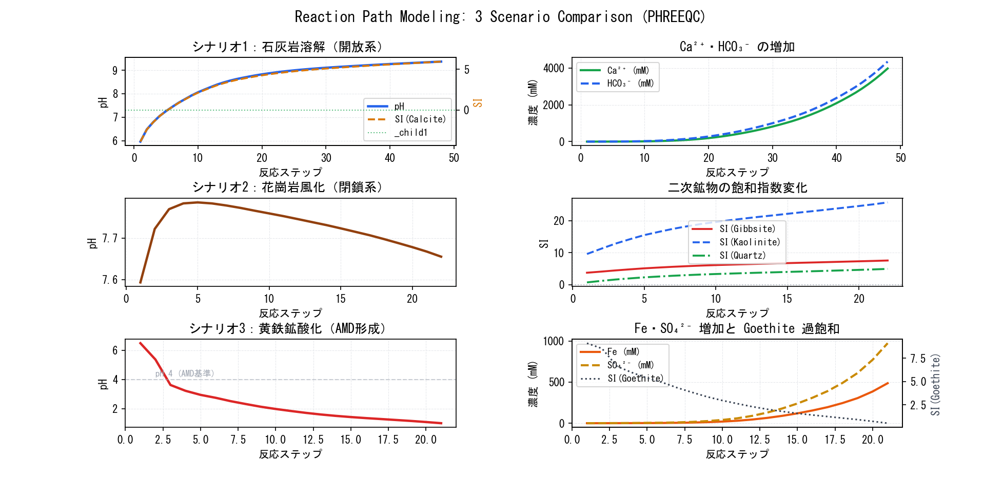
Discussion: What the 3 Scenarios Reveal
Figure 3. Comparison of pH Trajectories — Limestone climbs, Granite rises gently, and Pyrite crashes.
SI(Calcite) crosses 0 and spikes (≈ +5)
Ca²⁺ and HCO₃⁻ increase continuously.
Continuous CO₂ supply drives dissolution, leading to extreme thermodynamic supersaturation without hitting an equilibrium stopping point.
Kaolinite & Gibbsite remain highly supersaturated.
Quartz slowly approaches saturation.
Secondary minerals are strongly supersaturated, but actual precipitation in nature is kinetically limited, maintaining a non-equilibrium state for long periods.
Fe and SO₄²⁻ increase exponentially.
SI(Goethite) spikes early but drops later.
Autocatalysis by Fe³⁺ accelerates the reaction. Acid generation destroys buffering capacity, driving the system into extreme acidity.
Conclusion: Integrating the Entire Series
Using the TRANSPORT block, we will simulate how pollutants and dissolved constituents spread through an aquifer via advection (carried by flow) and dispersion (spreading out). This adds the dimension of “Space” to the reaction paths developed in Part 11!