Getting Started with PHREEQC #19: Specific Surface Area Pitfalls — Unit Mismatch and Physical Meaning of Calibration Factors

Introduction

In geochemical kinetic modeling using PHREEQC, one of the most problematic parameters for modelers is the specific surface area (SSA) of minerals.

In reactive transport codes such as TOUGHREACT or CrunchFlow, the input specific surface area is automatically converted to the absolute surface area under hydrological conditions by the internal calculation engine, taking mineral molecular weight and grid volume into account. However, since PHREEQC requires users to write their own rate equations (RATES block) using BASIC, this conversion must be handled manually by the modeler.

This requirement introduces several critical pitfalls. In this article, we demonstrate how common technical errors—such as unit mismatches and the omission of mineral molecular weight and initial mass—corrupt the physical meaning of calibration parameters. Furthermore, we address the fundamental limitation of the unmeasurable "reactive surface area (RSA)" and propose a rigorous practice for defining and reporting surface area settings in geochemical simulations.

1. Dimensional Analysis of Rate Equations: What "Aligning" \(k\) and \(A_s\) Means

The complete rate equation for mineral dissolution adopted by Lasaga et al. (1994) and Palandri & Kharaka (2004) is expressed as:

\[ r_{\mathrm{net}} = A_s \left[ k_{\mathrm{nu}} \exp\!\left(\frac{-E_{a,\mathrm{nu}}}{RT}\right) + k_H \exp\!\left(\frac{-E_{a,H}}{RT}\right) a_H^{n_H} + k_{\mathrm{OH}} \exp\!\left(\frac{-E_{a,\mathrm{OH}}}{RT}\right) a_{\mathrm{OH}}^{n_{\mathrm{OH}}} \right](1 - \Omega) \tag{1} \]

Where the units of each term are:

\(r_{\mathrm{net}}\): net reaction rate \([\mathrm{mol\,kgw^{-1}\,s^{-1}}]\)
\(A_s\): contact surface area per unit mass of water \([\mathrm{m^2\,kgw^{-1}}]\)
\(k_{\mathrm{nu}},\, k_H,\, k_{\mathrm{OH}}\): rate constants for each mechanism \([\mathrm{mol\,m^{-2}\,s^{-1}}]\)
\(E_a\): activation energy \([\mathrm{J\,mol^{-1}}]\)

Dimensional analysis yields:

\[ [A_s] \cdot [k] = \mathrm{m^2\,kgw^{-1}} \cdot \mathrm{mol\,m^{-2}\,s^{-1}} = \mathrm{mol\,kgw^{-1}\,s^{-1}} \quad \checkmark \]

Crucially, the area term \(\mathrm{m^{-2}}\) in the unit of \(k\) and the area term \(\mathrm{m^2}\) in \(A_s\) must represent the area measured by the exact same definition; otherwise, this multiplication loses its physical meaning. Because the rate constants of Palandri & Kharaka (2004) were normalized by the specific surface area measured via the BET method in laboratory experiments, the \(A_s\) input into PHREEQC must also be based on the BET definition.

2. Definitions and Conversions of Specific Surface Areas

2.1 Geometric Specific Surface Area (\(A_\mathrm{geo}\))

Assuming spherical particles with diameter \(d\,[\mathrm{m}]\) and density \(\rho\,[\mathrm{g/m^3}]\), the geometric surface area is defined as:

\[ A_\mathrm{geo} = \frac{6}{d \cdot \rho} \quad [\mathrm{m^2/g}] \tag{2} \]

For example, for quartz (\(\rho = 2.65 \times 10^6\,\mathrm{g/m^3}\)) with a grain size of \(d = 100\,\mu\mathrm{m}\) (\(1.0 \times 10^{-4}\,\mathrm{m}\)):

\[ A_\mathrm{geo} = \frac{6}{1.0 \times 10^{-4} \times 2.65 \times 10^6} \approx 0.023\,\mathrm{m^2/g} \]

This value serves as a lower-bound estimate that neglects mineral surface roughness and internal pores (Appelo & Postma, 2005).

2.2 BET Specific Surface Area (\(A_\mathrm{BET}\))

Calculated from gas adsorption isotherms under liquid nitrogen temperature (Brunauer et al., 1938), this method measures the total surface area accessible to gas molecules, incorporating fine surface roughness and pores. The ratio of \(A_\mathrm{BET}\) to \(A_\mathrm{geo}\) (roughness factor) is defined as:

\[ \lambda = \frac{A_\mathrm{BET}}{A_\mathrm{geo}} \tag{3} \]

White & Peterson (1990) reported \(\lambda \approx 7\) for fresh silicate minerals, though \(\lambda\) can range from 10 to 600 for highly weathered samples (White & Brantley, 2003).

2.3 Molar Specific Surface Area (\(A_\mathrm{mol}\))

Often used in PHREEQC databases. The relationship with \(A_\mathrm{BET}\) is:

\[ A_\mathrm{mol} = A_\mathrm{BET} \times M_w \quad [\mathrm{m^2/mol}] \tag{4} \]

2.4 PHREEQC Input: Final Conversion to \(\mathrm{m^2/kgw}\) and the "No-Error Trap"

This is the most common pitfall for beginners.

When writing moles = rate * area * TIME in the RATES block of PHREEQC, the unit of area must be \([\mathrm{m^2\,kgw^{-1}}]\) (total surface area per unit mass of water). However, beginners often input specific surface area values (e.g., \(A_\mathrm{BET} = 0.1\,\mathrm{m^2/g}\) or \(A_\mathrm{geo} = 0.023\,\mathrm{m^2/g}\)) directly into the area variable or as parameters (-parms) in the KINETICS block.

PHREEQC does not throw an error and computes plausible curves even with this unit mismatch.

If a specific surface area in \([\mathrm{m^2/g}]\) is directly assigned to area, the software implicitly assumes a special case where the mineral mass per unit water is exactly \(1\,\mathrm{g/kgw}\).

Consequently, severe computational errors occur without any warning from PHREEQC: - If the actual mineral mass is \(10\,\mathrm{g/kgw}\), the surface area should be 10 times larger (\(A_\mathrm{BET} \times 10\)). Assigning \(A_\mathrm{BET}\) directly underestimates the reaction rate by a factor of 10 (10-fold underestimation). - If the actual mineral mass is \(0.1\,\mathrm{g/kgw}\), the surface area should be 10 times smaller (\(A_\mathrm{BET} \times 0.1\)). Assigning \(A_\mathrm{BET}\) directly overestimates the reaction rate by a factor of 10 (10-fold overestimation).

To correctly convert the geometric specific surface area \(A_\mathrm{geo}\;[\mathrm{m^2/g}]\) into the dynamic surface area \(A_s(t)\;[\mathrm{m^2/kgw}]\) for PHREEQC, follow these three steps:

Step 1: Conversion to physical surface area considering surface roughness (\(\lambda\)): Multiply the geometric surface area \(A_\mathrm{geo}\;[\mathrm{m^2/g}]\) by the roughness factor \(\lambda\) to estimate the BET specific surface area \(A_\mathrm{BET}\;[\mathrm{m^2/g}]\). \[ A_\mathrm{BET}\;[\mathrm{m^2/g}] = A_\mathrm{geo}\;[\mathrm{m^2/g}] \times \lambda \]
Step 2: Conversion per unit water mass using initial mineral mass \(W(0)\;[\mathrm{g/kgw}\)]: Multiply the specific surface area \(A_\mathrm{BET}\) by the initial mineral mass per 1 kgw of water, \(W(0)\;[\mathrm{g/kgw}]\), to obtain the initial total surface area \(A_s(0)\;[\mathrm{m^2/kgw}]\). \[ A_s(0)\;[\mathrm{m^2/kgw}] = A_\mathrm{BET}\;[\mathrm{m^2/g}] \times W(0)\;[\mathrm{g/kgw}] \] Using the initial moles \(M(0)\;[\mathrm{mol/kgw}]\) and molecular weight \(M_w\;[\mathrm{g/mol}]\), the initial mass is expressed as \(W(0) = M(0) \times M_w\). Therefore, the equation is simplified to: \[ A_s(0) = A_\mathrm{BET} \times M_w \times M(0) \tag{5} \]
Step 3: Dynamic modeling of surface area changes during dissolution: As dissolution progresses, the mineral volume and surface area decrease. If we adopt the Shrinking Core Model (assuming uniform dissolution of spherical particles), the surface area decreases in proportion to the 2/3 power of the remaining molar ratio. With the current moles denoted as \(M(t)\), the current surface area \(A_s(t)\;[\mathrm{m^2/kgw}]\) is dynamically computed as: \[ A_s(t) = A_s(0) \times \left(\frac{M(t)}{M(0)}\right)^{2/3} = A_\mathrm{BET} \times M_w \times M(0) \times \left(\frac{M(t)}{M(0)}\right)^{2/3} \tag{6} \]

3. Critical Pitfall: Omission of Molecular Weight and Initial Mass, and the Collapse of Calibration Parameter Meaning

In PHREEQC manuals and sample codes, the following expression is frequently encountered:

area = area_init * (M/M_init)^(2/3)

In many cases, modelers substitute the specific surface area \([\mathrm{m^2/g}]\) directly into area_init, completely omitting the molecular weight \(M_w\) and the initial moles \(M(0)\).

This omission results in the incorrect surface area calculation shown below:

\[ A_{s,\mathrm{wrong}}(t) = A_\mathrm{BET} \times \left(\frac{M(t)}{M(0)}\right)^{2/3} \tag{7} \]

Comparing this with the correct expression in Equation (6), the term for the initial mineral mass \(W(0) = M(0) \times M_w\) is completely lost.

If a modeler calibrates this incorrect model to match experimental data by adjusting a scaling factor (\(f_\mathrm{fit}\)), the relationship between the incorrect calibration factor \(f_{\mathrm{fit},\mathrm{wrong}}\) and the correct factor \(f_{\mathrm{fit},\mathrm{correct}}\) becomes:

\[ f_{\mathrm{fit},\mathrm{wrong}} = f_{\mathrm{fit},\mathrm{correct}} \times W(0) \tag{8} \]

This reveals a fatal consequence: even for the same mineral under identical flow conditions, the calibrated parameter value will shift by orders of magnitude depending on the initial mineral mass \(W(0)\) used in the experiment.

For example, if one experiment uses \(10\,\mathrm{g/kgw}\) of quartz and another uses \(0.1\,\mathrm{g/kgw}\), using the code that omits molecular weight will introduce a 100-fold discrepancy in the calibrated parameter values.

This completely destroys the physical meaning (e.g., reactive site density or hydrological effects) that the calibration parameter should represent. The parameter is reduced to a "meaningless number (fudge factor) that merely absorbs the omission of initial mass and molecular weight for that specific experimental setup." This omission is the primary technical reason why calibrated parameters vary wildly between researchers and experimental systems, preventing any meaningful comparison.

4. Quantitative Impact of Surface Area Mismatch on Dissolution Calculations

When \(A_\mathrm{geo}\) is directly input instead of the BET-based area, or when the molecular weight is omitted, the discrepancy between the calculated and true reaction rates spans several orders of magnitude due to the roughness factor \(\lambda\) and initial mass \(W(0)\).

The following simulation demonstrates the impact of definition mismatch and conversion omission on the dissolution of Albite at 25°C over one year.

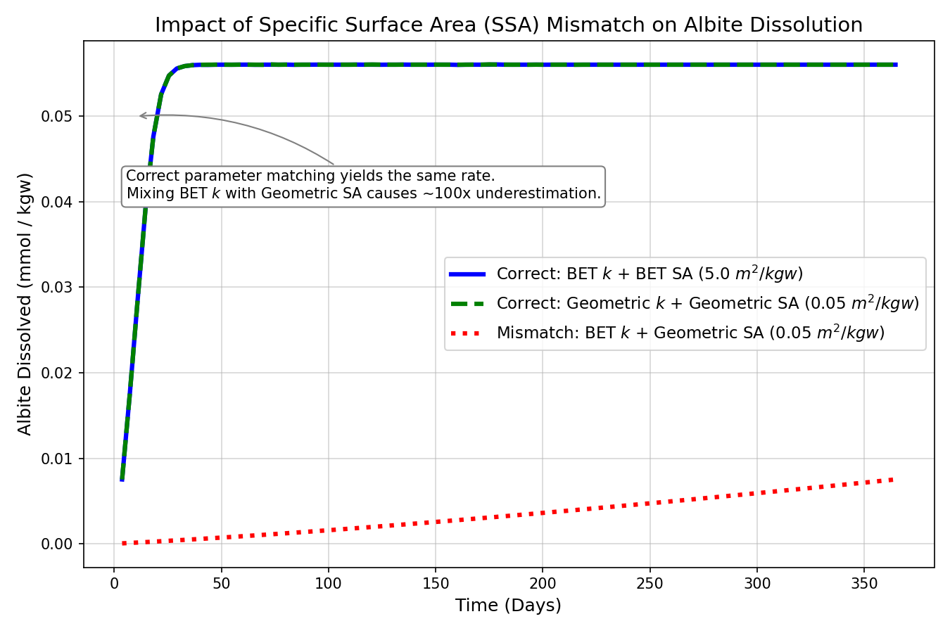
Impact of specific surface area definition mismatch on dissolution amount

The system combining the BET-based \(k\) and the correctly converted BET area (blue line) perfectly matches the system combining the geometric area (Geo) and the geometric-based rate constant \(k_{\mathrm{geo}}\) (\(= \lambda \cdot k_{\mathrm{BET}}\)) (green line).

Although the geometric-based rate constant is theoretically defined as \(k_{\mathrm{geo}} = \lambda \cdot k_{\mathrm{BET}}\), in modeling practice, standard rate constant databases (such as Palandri & Kharaka, 2004) are consistently normalized to the BET baseline. Consequently, geometric-based rate constants do not exist in standard databases.

Therefore, if a modeler inputs the geometric surface area \(A_{\mathrm{geo}}\) while directly using the database’s \(k_{\mathrm{BET}}\), it inevitably introduces a \(\lambda\)-fold definition mismatch (red line, where \(\lambda = 100\)). When fitting a model using the geometric area, one must be aware that the resulting scaling factor automatically absorbs the influence of the roughness factor \(\lambda\) (ranging from several times to hundreds of times) from the very beginning.

5. Geochemical Limitation: The Unmeasurable "Reactive Surface Area (RSA)"

Even if the technical unit conversions and molecular weight inputs are handled correctly, modelers face a more fundamental scientific limitation.

The rate equations require neither the gas-accessible area (\(A_\mathrm{BET}\)) nor the smooth geometric area (\(A_\mathrm{geo}\)), but the surface area actively reacting with water, known as the "Reactive Surface Area (RSA)." Currently, RSA cannot be measured directly. The relationship between these area concepts is conceptualized as follows:

\[ A_\mathrm{geo} \xrightarrow{+\,\text{surface roughness}} A_\mathrm{BET} \xrightarrow{+\,\text{reactive heterogeneity}} A_\mathrm{RSA} \xleftarrow{-\,\text{model errors, etc.}} A_\mathrm{eff} \]

While the transition from \(A_\mathrm{geo}\) to \(A_\mathrm{BET}\) is quantified via the roughness factor \(\lambda\), the path from \(A_\mathrm{BET}\) to the true \(A_\mathrm{RSA}\) remains unquantifiable.

Several studies highlight the limitations of the BET method:

Non-proportionality of BET area and dissolution rate: Gautier et al. (2001) observed that during quartz dissolution, the dissolution rate remained constant despite a continuous increase in the BET area, suggesting that internal pores do not participate in the reaction.
Responsibility transfer to surface area: Maher (2010) explained the orders-of-magnitude discrepancy between laboratory and field weathering rates as a consequence of fluid residence time and thermodynamic saturation state. From this perspective, adjusting the surface area parameter to fit data simply transfers the responsibility of unrepresented physical processes (e.g., heterogeneous flow fields and residence time distributions) to the surface area.
Limitations of a single parameter: Lüttge and coworkers pointed out that mineral surface reactivity is highly heterogeneous due to crystal defects and etch pits, meaning that representing it with a single average rate constant or surface area is physically limited (Fischer et al., 2012).

Regardless of how precisely we measure specific surface area, the calibrated effective surface area \(A_\mathrm{eff}\) inevitably acts as a sink for unrepresented physical and chemical errors within the model.

6. Practical Proposals: Equivalence and Transparent Reporting of Calibration Factors

Consequently, the calibrated scaling factor \(f_{\mathrm{fit}}\) is not a physical correction for the surface area. Instead, it is a "Coupled Effective Parameter" that aggregates the effects of transport heterogeneity, thermodynamic database errors, and surface reactivity variations.

Because the aggregated errors and experimental conditions differ between systems, it is natural that calibrated values vary across studies. To address this, modelers should adopt the following practices:

Use equations that correctly incorporate molecular weight and initial mineral mass Eliminate the dependency on the initial mass \(W(0)\), ensuring that parameters remain physically comparable across experiments with different mineral loadings.
Transparently report the calibration factor \(f_{\mathrm{fit}}\) and its baseline When scaling the surface area, report the exact scaling factor \(f_{\mathrm{fit}}\) along with the definition of the baseline area (e.g., \(A_\mathrm{geo}\) calculated from grain size or \(A_\mathrm{BET}\) with gas type specified).

7. Correct PHREEQC Implementation and Case Studies

7.1 Basic Implementation Template

The following BASIC code demonstrates how to avoid manual pre-calculations and dynamically convert the specific surface area \([\mathrm{m^2/g}]\) to \([\mathrm{m^2/kgw}]\) within PHREEQC:

# ===== Dynamic Conversion from Specific Surface Area and Implementation of Calibration Factor =====
# A_ref : Reference specific surface area A_geo = 0.023 m2/g (grain size 100 um)
# f_fit : Calibration scaling factor (dimensionless)
#         *Note: This is a coupled effective parameter absorbing unrepresented
#                model errors, not a pure physical surface area.

10 m_init = PARM(1)        # Initial moles (mol/kgw)
20 Mw     = 262.22         # Mineral molecular weight (g/mol)
30 A_ref  = PARM(2)        # Reference specific surface area (m2/g)
40 f_fit  = PARM(3)        # Scaling factor (e.g., 0.01)
50 m_curr = M
60 IF (m_curr <= 0) THEN GOTO 200

# Dynamically convert to m2/kgw by multiplying Mw and m_init, then apply f_fit
70 area   = A_ref * f_fit * Mw * m_init * (m_curr / m_init)^(2/3)  # m2/kgw
80 moles  = rate * area * TIME
90 SAVE moles
100 END
200 SAVE 0

In the KINETICS block, parameters are passed as follows:

KINETICS 1
    Mineral_Phase
        -m 0.0263
        -parms 0.0263 0.023 0.01   # m_init, A_ref(m2/g), f_fit

7.2 Case Studies: Redesigning Codes from Series #17 and #18

The codes presented in our previous posts, "#17: Challenging Basalt-CO2 Reactions (CarbFix)" and "#18: Reproducing Rishiri Basalt Batch Experiments," relied on manual pre-calculations. This design made the BASIC codes incomplete on their own and prone to user errors when copied. Below, we redesign these models.

Case 1: Redesigning Series #17 (Basaltic Glass Dissolution)

Before correction (manual pre-calculation): The KINETICS block passed -parms 1.255 37500. The value 37500 was calculated manually by multiplying the specific surface area \(250\,\mathrm{m^2/g}\) by the initial glass mass \(150\,\mathrm{g}\) (\(250 \times 150 = 37500\)). The RATES block computed the area as:
```
110 m_init = PARM(1)
120 s_init = PARM(2)
130 m_curr = M
150 current_S = s_init * (m_curr / m_init)^(2/3)
```

After correction (dynamic conversion within code): We pass the specific surface area \(250.0\) (\(\mathrm{m^2/g}\)) directly via PARM(2). The molecular weight of the basaltic glass (\(Mw = 119.52\,\mathrm{g/mol}\)) is hardcoded.

To verify mathematical equivalence, the dynamic initial surface area is calculated as: \[ A_{\mathrm{BET}} \times M_w \times M(0) = 250.0 \times 119.52 \times 1.255 \approx 37500.12 \] This matches the manual value of \(37500\) with high precision, yielding identical results.

# KINETICS block
Basalt_Glass
    -m 1.255
    -parms 1.255 250.0  # m_init, A_BET(m2/g) specified directly

# RATES block
# (omitted: calculation of rate constant k, etc.)
110 m_init = PARM(1)
120 A_BET  = PARM(2)       # Specific surface area 250.0 m2/g
125 Mw     = 119.52        # Basaltic glass molecular weight (g/mol)
130 m_curr = M
140 IF (m_curr <= 0) THEN GOTO 200
# Dynamically convert to m2/kgw within the code
150 current_S = A_BET * Mw * m_init * (m_curr / m_init)^(2/3)
160 rate_mol = specific_rate * current_S
170 moles = rate_mol * TIME
180 SAVE moles
190 END
200 SAVE 0

Case 2: Redesigning Series #18 (Rishiri Basalt Batch / Albite Dissolution)

Before correction (manual pre-calculation): The KINETICS block passed -parms 0.0263 0.0526. The value 0.0526 was calculated manually by multiplying the geometric area \(2.63\,\mathrm{m^2}\) (derived from initial mass \(6.90\,\mathrm{g}\)) by the reactive surface area ratio (RSA = 2%). The RATES block computed the area as:
```
50 m_init = PARM(1)
60 area_init = PARM(2)
70 m_curr = M
90 area = area_init * (m_curr / m_init)^(2/3)
```

After correction (dynamic conversion within code): We pass the geometric specific surface area \(A_{\mathrm{geo}} = 0.3817\,\mathrm{m^2/g}\) via PARM(2) and the effective scaling factor (RSA = 2% = 0.02) via PARM(3). The molecular weight of Albite (\(262.22\,\mathrm{g/mol}\)) is used.

Verifying equivalence, the dynamic initial surface area is: \[ A_{\mathrm{geo}} \times f_{\mathrm{fit}} \times M_w \times M(0) = 0.3817 \times 0.02 \times 262.22 \times 0.0263 \approx 0.05264 \] This matches the manual value of \(0.0526\) down to four decimal places, generating identical dissolution curves.

# KINETICS block
Albite(low)
    -m 0.0263
    -parms 0.0263 0.3817 0.02   # m_init, A_geo(m2/g), f_fit(RSA)

# RATES block
# (omitted: calculation of rate constant k, etc.)
50 m_init = PARM(1)
60 A_geo  = PARM(2)       # Geometric specific surface area 0.3817 m2/g
65 f_fit  = PARM(3)       # Calibration factor (RSA = 0.02)
68 Mw     = 262.22        # Albite molecular weight (g/mol)
70 m_curr = M
80 IF (m_curr <= 0) THEN GOTO 200
# Convert to m2/kgw dynamically
90 area   = A_geo * f_fit * Mw * m_init * (m_curr / m_init)^(2/3)
100 moles = rate * area * TIME
110 SAVE moles
120 END
200 SAVE 0

Redesigning the parameter structure eliminates the need for manual pre-calculations in the KINETICS block, yielding a self-explanatory model that clearly documents the surface area scaling ratio.

8. Conclusion: Dimensional Rigor and Honest Reporting of Limitations

In geochemical kinetic modeling, calibrating surface area parameters is an inevitable practice. However, calibrations performed with incomplete codes that omit molecular weights and initial masses produce parameters that cannot be compared across systems.

Modelers must perform correct dimensional conversions, eliminate initial mass dependencies, and honestly report the limitations of calibrated parameters as "effective coupled variables." This transparent approach is essential to prevent the misinterpretation of fitted parameters as physical truths.

References

Appelo, C. A. J., & Postma, D. (2005). Geochemistry, groundwater and pollution (2nd ed.). CRC press.
Brantley, S. L., & Mellott, N. P. (2000). Surface area and porosity of primary silicate minerals. American Mineralogist, 85(11–12), 1767–1783.
Brunauer, S., Emmett, P. H., & Teller, E. (1938). Adsorption of gases in multimolecular layers. Journal of the American Chemical Society, 60(2), 309–319.
Fischer, C., Arvidson, R. S., & Lüttge, A. (2012). How predictable are dissolution rates of crystalline material? Geochimica et Cosmochimica Acta, 98, 177-185.
Gautier, J. M., Oelkers, E. H., & Schott, J. (2001). Are quartz dissolution rates proportional to B.E.T. surface areas? Geochimica et Cosmochimica Acta, 65(7), 1059-1070.
Hodson, M. E., Langan, S. J., & Meriau, S. (2006). Does reactive surface area depend on grain size? Geochimica et Cosmochimica Acta, 70(7), 1670–1687.
Lasaga, A. C., Soler, J. M., Ganor, J., Burch, T. E., & Nagy, K. L. (1994). Chemical weathering rate laws and global geochemical cycles. Geochimica et Cosmochimica Acta, 58(10), 2361–2386.
Maher, K. (2010). The dependence of chemical weathering rates on fluid residence time. Earth and Planetary Science Letters, 294(1-2), 101-110.
Palandri, J. L., & Kharaka, Y. K. (2004). A compilation of rate parameters of water-mineral interaction kinetics for application to geochemical modeling. USGS Open-File Report 2004-1068.
White, A. F., & Brantley, S. L. (2003). The effect of time on the weathering of silicate minerals: why do weathering rates differ in the laboratory and field? Chemical Geology, 202(3–4), 479–506.
White, A. F., & Peterson, M. L. (1990). Role of reactive-surface-area characterization in geochemical kinetic models. ACS Symposium Series, 416, 461–475.

Note: The explanation of physical unit conversions and the redesign of the PHREEQC code in this article were prepared and organized with the assistance of AI (Gemini and Claude).