1 Introduction: The True Meaning of “Elevation” on a Contour Map
In Part 2, we learned that groundwater is stored within the geological “vessel” and flows slowly, driven by the undulations of the land surface.
But have you ever looked at a groundwater contour map? It shows “elevations” much like a topographic map of mountains — but what exactly do these “elevations” represent? They are not the altitude of mountains. And why does groundwater move in a particular direction, at a particular speed?
In Part 3, we confront the most fundamental physical law governing groundwater flow: Darcy’s Law. In 1856, a French engineer named Henri Darcy discovered this law through a simple experiment of flowing water through a column of sand. Its elegant simplicity remains the starting point for all modern groundwater modeling.
2 Forms of Groundwater: Saturated and Unsaturated Zones
First, is all water beneath the surface “groundwater”? Actually, no. Imagine a vertical cross-section from the ground surface downward.
2.1 The Unsaturated Zone (Vadose Zone)
The section from the ground surface down to the water table is called the unsaturated zone. In this region, soil pores contain a mixture of water and air. Water is held not only by gravity but also by capillary pressure — the attractive force generated by the surface tension of liquid water and the wettability of solid surfaces(Freeze and Cherry 1979). It is the same principle by which a dry sponge or tissue paper absorbs water.
Flow in the unsaturated zone behaves fundamentally differently from the saturated zone. As the water saturation \(S_w\) decreases, the effective pathways available for water diminish, causing the water’s ability to flow (relative permeability \(k_r\)) to drop sharply. At a certain saturation (the residual saturation), water can no longer move(登坂 2006). Such multiphase flow is described by the generalized Darcy’s law or the Richards equation — details reserved for Part 8 (Recharge Processes).
2.2 The Saturated Zone
Below the water table lies the saturated zone, where pores are 100% filled with water and no air exists. What we commonly call “groundwater” refers to water in this zone. Analysis of flow in the saturated zone is the central theme of groundwater science, and Darcy’s Law is precisely the law governing this domain.
Porosity (\(n\)) is the ratio of void volume to total rock volume. In sedimentary rocks, it varies widely from 10 to 50%, while in igneous and metamorphic rocks, fractures serve as the main void space(Freeze and Cherry 1979). Within the pore space, water (liquid phase) and gas (gas phase) coexist, and their respective fractions are called water saturation \(S_w\) and gas saturation \(S_g\) (\(S_w + S_g = 1\)). In the saturated zone, \(S_w = 1\).
3 Bernoulli’s Theorem and Total Head
The driving force behind groundwater flow is the natural principle that “water flows from higher energy to lower energy.” Bernoulli’s theorem, the energy conservation law of fluid dynamics, applies to groundwater as well.
Total Head (\(h\)) is expressed as the sum of three components:
\[h = z + \frac{P}{\rho g} + \frac{v^2}{2g} \tag{1}\]
- Elevation Head (\(z\)): Potential energy due to height above a datum
- Pressure Head (\(P/\rho g\)): Energy due to water pressure
- Velocity Head (\(v^2/2g\)): Kinetic energy of the water
Here, a key characteristic of groundwater flow comes into play. Groundwater velocity is extremely slow — typically ranging from a few cm/day to a few m/day. Substituting these velocities into Equation 1, the velocity head \(v^2/2g\) becomes more than seven orders of magnitude smaller than the other terms.
Therefore, in groundwater flow, velocity head can be neglected, and total head is effectively simplified as(Freeze and Cherry 1979):
\[h = z + \frac{P}{\rho g} \tag{2}\]
The water level measured in a well (piezometric head) represents exactly this total head. The “elevation” drawn on groundwater contour maps is the sum of potential energy and pressure energy expressed as the height of a water column — that is, the total head.
4 Types of Aquifers: Unconfined and Confined
Geological formations that transmit water easily are called aquifers. We touched on this in Part 2, but here we will go deeper, understanding them from the perspective of the conversion mechanism between pressure head and elevation head.
4.1 Unconfined Aquifer
An aquifer without an impermeable layer (cap) above it, allowing the water table to fluctuate freely. The water level in a well corresponds directly to the water table. At the water table, pressure equals atmospheric pressure (gauge pressure = zero), so the water level equals the elevation of the water table.
4.2 Confined Aquifer
An aquifer sandwiched between impermeable layers above and below. The water is trapped under pressure. When a well is drilled, water rises above the confining layer. The imaginary surface that this water level reaches is called the potentiometric surface.
What matters in a confined aquifer is the conversion between pressure head and elevation head in the total head equation (Equation 2). At the aquifer’s deep position, elevation head \(z\) is small, but pressure head \(P/\rho g\) is large due to confinement. Drilling a well releases this pressure energy, causing water to rise — this is the confined mechanism.
Furthermore, if the potentiometric surface exceeds the ground surface, water will flow out of the well on its own — creating an artesian well. A confined groundwater system can be understood by analogy with a municipal water supply. A water tower at a high elevation (recharge area) pressurizes water in the pipe, and opening a faucet (well) at a lower elevation allows water to flow out — the principle is the same.
Artesian wells have two possible states. When the potentiometric surface is below the ground surface, water does not reach the surface naturally, and pumping is required (non-flowing artesian well). Only when the potentiometric surface is above the ground surface does spontaneous flow occur (flowing artesian well). Note that “confined” does not automatically mean “flowing.”
5 Darcy’s Law
Now we arrive at the most important law in groundwater science.
In 1856, French engineer Henri Darcy, working to improve the water supply system of the city of Dijon, conducted experiments flowing water through a vertical column packed with sand. He discovered that the flow rate is proportional to the “ease of water transmission” (hydraulic conductivity) and the “difference in water levels” (hydraulic gradient)(Freeze and Cherry 1979; Yamamoto 1983).
\[Q = -K \cdot A \cdot \frac{\Delta h}{\Delta l} \tag{3}\]
- \(Q\): Volumetric flow rate (\(m^3/day\))
- \(K\): Hydraulic Conductivity (\(m/day\)) — the aquifer’s ability to transmit water
- \(A\): Cross-sectional area (\(m^2\))
- \(\frac{\Delta h}{\Delta l}\): Hydraulic Gradient (dimensionless)
The negative sign indicates that water flows from higher to lower head. The specific discharge (Darcy flux) \(q\), obtained by dividing by the cross-sectional area \(A\):
\[q = -K \frac{dh}{dl} \tag{4}\]
Darcy flux \(q\) uses the entire cross-section (solid + pores) as the denominator, making it an “apparent velocity.” The actual velocity at which water passes through the pores (seepage velocity) is \(v = q / n\) (where \(n\) is the effective porosity), which is larger than Darcy flux. Seepage velocity is what matters when considering contaminant transport rates.
5.1 Hydraulic Conductivity \(K\) and Intrinsic Permeability \(k\)
Darcy’s Law appears simple, but note that hydraulic conductivity \(K\) incorporates both properties of the geological formation and the fluid(登坂 2006):
\[K = \frac{k \rho g}{\mu} \tag{5}\]
- \(k\): Intrinsic Permeability (\(m^2\)) — formation-specific transmissibility (independent of the fluid)
- \(\rho\): Fluid density (\(kg/m^3\))
- \(\mu\): Dynamic viscosity (\(Pa \cdot s\))
- \(g\): Gravitational acceleration (\(m/s^2\))
This means that for the same aquifer, hydraulic conductivity changes depending on whether the flowing liquid is fresh water, oil, or thermal spring water. In petroleum engineering and geochemical modeling, intrinsic permeability \(k\) is used, while in hydrogeology, hydraulic conductivity \(K\) is the standard(Freeze and Cherry 1979).
When extending Darcy’s Law to other fluids or the unsaturated zone, relative permeability \(k_r(S_w)\) — a function of saturation — is multiplied with intrinsic permeability \(k\), yielding the generalized Darcy’s law, a more general description of fluid flow that encompasses Equation 4.
5.2 Analogous Laws: Empirical Laws with the Same Mathematical Form
The beauty of Darcy’s Law lies in its mathematical form being isomorphic to other physical laws(登坂 2006):
| Law | Physical Quantity | Driving Force | “Ease” of Transport |
|---|---|---|---|
| Darcy’s Law | Water flow | Hydraulic head difference | Hydraulic conductivity \(K\) |
| Fourier’s Law | Heat conduction | Temperature difference | Thermal conductivity \(\lambda\) |
| Fick’s Law | Mass diffusion | Concentration difference | Diffusion coefficient \(D\) |
| Ohm’s Law | Electric current | Potential difference | Electrical conductivity \(\sigma\) |
“Flux = coefficient × gradient of driving force” — this simple structure appears repeatedly across all scales of the natural world.
6 Experiencing Theory with a 1D Darcy Model
Having learned the theory, let’s build a real model using MODFLOW 6 and Python (FloPy) to “numerically experience” Darcy’s Law.
flopy is a Python wrapper library, and the actual computation requires the MODFLOW 6 executable (mf6 or mf6.exe) separately. Download it from the USGS official website and either add it to your PATH or place it in the working directory.
6.1 Model Setup
- A 1D column 100 m long (10 cells of 10 m × 10 m)
- Hydraulic Conductivity \(K\) = 10 m/day
- Head at the left end (col 0) = Fixed at 10 m
- Head at the right end (col 9) = Fixed at 5 m
6.2 Manual Calculation
Substituting values into Equation 4:
\[q = -K \frac{\Delta h}{\Delta l} = -10 \times \frac{5 - 10}{100} = 0.5 \text{ m/day}\]
We verify this with FloPy. However, an important caveat exists when precisely comparing this manual calculation with MODFLOW’s numerical solution.
6.3 Modeling with FloPy
The following code builds and runs the model to verify the head distribution.
Show FloPy model code
import flopy
import numpy as np
from pathlib import Path

name = "darcy_1d"
ws = Path("./model_ws").resolve()
ws.mkdir(exist_ok=True)
sim = flopy.mf6.MFSimulation(sim_name=name, sim_ws=str(ws), exe_name="mf6")

# Steady-state
tdis = flopy.mf6.ModflowTdis(sim, time_units="DAYS", perioddata=[(1.0, 1, 1.0)])
ims = flopy.mf6.ModflowIms(sim, complexity="SIMPLE")
gwf = flopy.mf6.ModflowGwf(sim, modelname=name, save_flows=True)

# Spatial discretization: 100m divided into 10 cells
dis = flopy.mf6.ModflowGwfdis(
    gwf, nlay=1, nrow=1, ncol=10,
    delr=10.0, delc=10.0, top=15.0, botm=0.0,
)

npf = flopy.mf6.ModflowGwfnpf(gwf, k=10.0)
ic = flopy.mf6.ModflowGwfic(gwf, strt=10.0)

# Constant Head (CHD): Left end 10m, Right end 5m
chd_spd = [[(0, 0, 0), 10.0], [(0, 0, 9), 5.0]]
chd = flopy.mf6.ModflowGwfchd(gwf, stress_period_data=chd_spd, save_flows=True)

oc = flopy.mf6.ModflowGwfoc(
    gwf,
    head_filerecord=f"{name}.hds",
    budget_filerecord=f"{name}.cbc",
    saverecord=[("HEAD", "ALL"), ("BUDGET", "ALL")],
)

sim.write_simulation()
success, buff = sim.run_simulation()
Visualizing the output head distribution yields Figure 1.
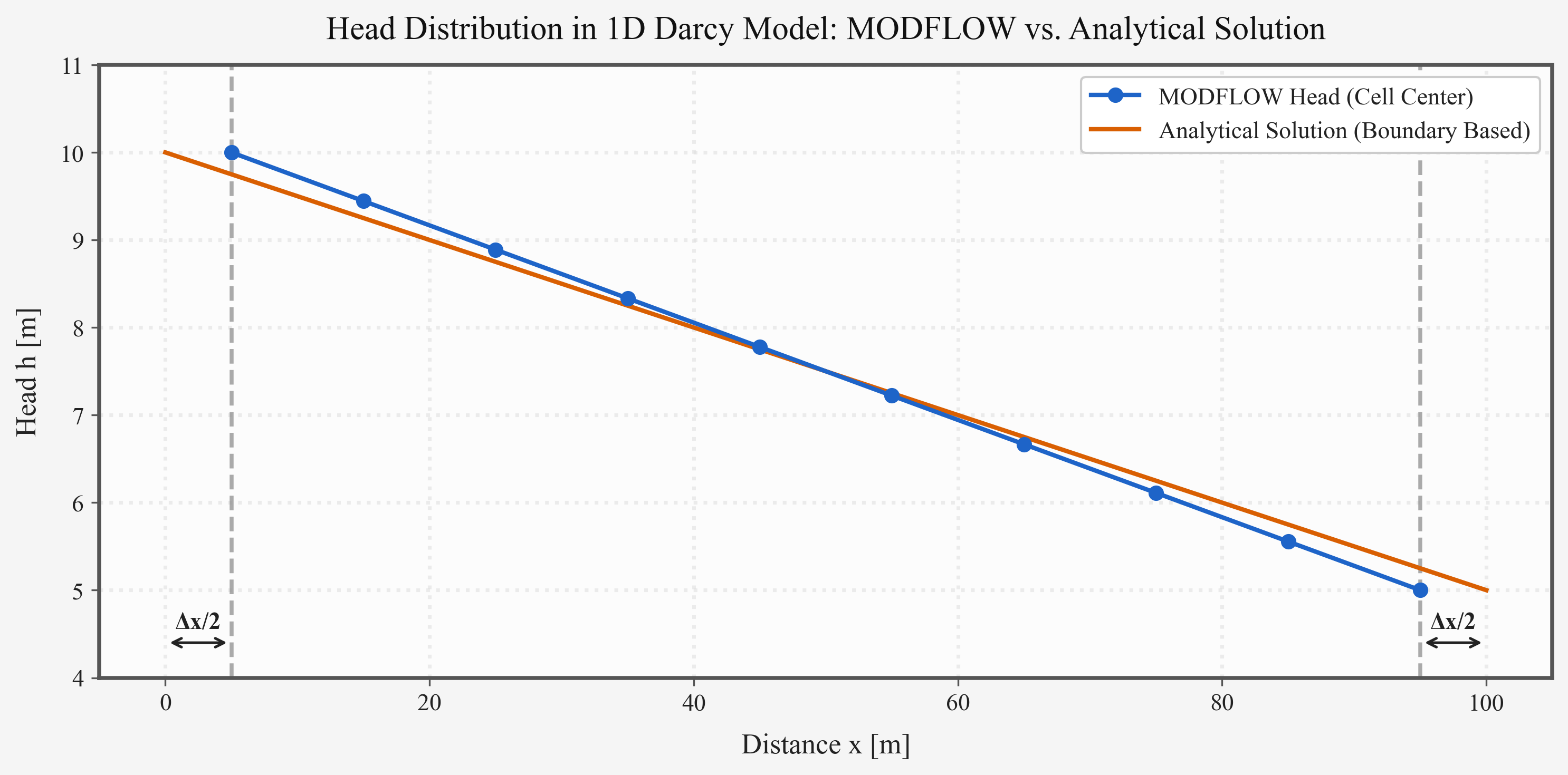
6.4 [Important] CHD Applies Head to the Cell Center
Looking closely at Figure 1, you can see that the MODFLOW points (blue) and the analytical solution line (orange dashed) are slightly offset. This is the exact point where one always stumbles when comparing numerical models to hand calculations.
MODFLOW 6’s CHD (Constant Head) package is designed to apply a constant head to the cell itself, not to the “boundary surface.” This means the head is defined at the physical center of the cell.
- Cell center of col 0: \(x = 5\) m ← \(h = 10\) m is applied
- Cell center of col 9: \(x = 95\) m ← \(h = 5\) m is applied
The “actual column length” of this model is 100 m, but the head boundary condition spans from \(x = 5\) m to \(x = 95\) m, i.e., over a distance of 90 m.
| Distance Δl | Specific Discharge q | |
|---|---|---|
| Manual Calculation (Analytical) | 100 m (Total column length) | −10 × (−5/100) = 0.500 m/day |
| MODFLOW Numerical Solution | 90 m (Between cell centers) | −10 × (−5/90) ≈ 0.556 m/day |
The difference is about 11%. This is called Spatial Discretization Error. As cells are subdivided, the cell center approaches the boundary surface, and the numerical solution converges to the analytical solution (spatial convergence).
When comparing numerical models to analytical solutions, always verify “where the boundary conditions are placed.” This is a critical concept common to all numerical methods: finite difference, finite element, and beyond. Increasing cell count by 10× reduces discretization error by approximately 1/10.
7 Conclusion
In Part 3, we learned the physical laws at the heart of groundwater science and how to verify them numerically.
- In the unsaturated zone, water and air coexist, and capillary pressure and relative permeability govern flow
- Total head \(h = z + P/\rho g\) is the driving force of groundwater flow; velocity head is negligible
- Water in confined aquifers rises through the conversion of pressure head to elevation head (the artesian well principle)
- Darcy’s Law \(q = -K \, dh/dl\) is the most fundamental equation describing saturated zone flow
- Hydraulic conductivity \(K\) incorporates both formation and fluid properties (\(K = k\rho g / \mu\))
- MODFLOW’s boundary condition (CHD) is defined at the cell center, requiring consideration of spatial discretization error when comparing to analytical solutions
8 Next Time
Part 4: Pumping Tests and Well Modeling.
What happens to groundwater when we pump from a well? We step beyond steady state into the world of transient flow. The Theis non-equilibrium equation, the cone of depression, and methods for estimating aquifer parameters from well test data.