In Episode 3, we learned about Darcy’s Law and the physics of head in steady-state conditions to understand which way and how fast groundwater moves.
In this episode, we will explore one of the most important field tests in groundwater development and environmental surveys: the Pumping Test, and the theory of Transient Flow behind it.
Although there are some math formulas, just like in Episode 3, they aren’t too difficult if we follow their meaning step by step. We’ll use Python visualizations to build an intuitive understanding.
1 Introduction: Like Sucking Water Through a Straw
Have you ever noticed how the surface of a drink dips slightly around a straw when you suck up the liquid vigorously?
When you pump groundwater from a well, the exact same thing happens underground. The water pressure around the well drops, and the water table forms a funnel-like shape. This shape of lowered water levels is called a Cone of Depression.
As pumping continues, this cone gradually expands outward and deepens over time. A flow where the state (like water level) keeps changing over time is called Transient Flow.
2 How Do We Measure Aquifer Properties? (Lab vs. Field Tests)
Why do hydrogeologists spend so much money and effort to conduct large-scale “pumping tests”? To deeply understand the reason, let’s compare them with small-scale indoor experiments (laboratory permeability tests).
2.1 Darcy’s Experiment: Constant-Head Test
The apparatus Darcy used, which we learned about in Episode 3, is still widely used today as the Constant-head test. By continuously supplying water at a constant head and measuring the volume of water passing through a cylindrical sand sample, we can calculate the soil’s “ability to transmit water” (Hydraulic Conductivity \(K\)). Because the water level does not change, this is an experiment of Steady Flow.
2.2 Water Level Drops Over Time: Falling-Head Test
On the other hand, for soils that don’t let water pass easily, like clay or silt, the Falling-head test is often used. In this test, a narrow pipe (standpipe) is filled with water, and we measure how fast the water level drops as it slowly seeps through the soil sample.
Because the water level changes over time, this is the simplest example of Transient Flow.
In an actual laboratory test, the Saturated Hydraulic Conductivity \(K\) is calculated using the following formula:
\[ K = \frac{2.3 \cdot a \cdot L}{A \cdot t} \log_{10} \frac{h_1}{h_2} \quad (\text{cm/sec}) \]
Here, the variables are defined as:
- \(a\): Cross-sectional area of the standpipe (\(\text{cm}^2\))
- \(A\): Cross-sectional area of the soil sample (\(\text{cm}^2\))
- \(L\): Length of the soil sample (\(\text{cm}\))
- \(t\): Measurement time (\(\text{sec}\))
- \(h_1\): Initial water level (height from the bottom of the sample) (\(\text{cm}\))
- \(h_2\): Final water level (height from the bottom of the sample) (\(\text{cm}\))
2.2.1 Temperature Correction for Hydraulic Conductivity (15°C)
Furthermore, the ability of water to flow is influenced by its viscosity, meaning the hydraulic conductivity changes with water temperature. Therefore, it is standard practice to correct the measured value to a standard temperature, typically 15°C (\(K_{15}\)).
\[ K_{15} = K_T \times \frac{\eta_T}{\eta_{15}} \]
- \(K_T\): Hydraulic conductivity at temperature \(T\)°C
- \(\eta_T\): Viscosity of water at temperature \(T\)°C
- \(\eta_{15}\): Viscosity of water at 15°C
The viscosity of water \(\eta_T\) at a given temperature \(W_t\) (°C) can be accurately estimated using the following empirical formula:
\[ \eta_T = \frac{100}{2.1482 \left[ (W_t - 8.435) + \sqrt{8078.4 + (W_t - 8.435)^2} \right] - 120} \]
2.2.2 Calculation Example
To make it easier to grasp, let’s manually calculate the hydraulic conductivity using actual laboratory dimensions.
[Measurement Conditions (Example)] - Standpipe cross-sectional area \(a = 0.503 \, \text{cm}^2\) - Sample cross-sectional area \(A = 19.6 \, \text{cm}^2\) - Sample length \(L = 5.1 \, \text{cm}\) - Initial water level \(h_1 = 18.0 \, \text{cm}\) - Final water level (after 360 seconds) \(h_2 = 8.0 \, \text{cm}\) - Measurement time \(t = 360 \, \text{sec}\) (6 minutes) - Water temperature \(W_t = 20 \, \text{°C}\)
1. Calculating Saturated Hydraulic Conductivity \(K_{20}\) First, we substitute the measured values into the formula:
\[ \begin{align*} K_{20} &= \frac{2.3 \times 0.503 \times 5.1}{19.6 \times 360} \log_{10} \left( \frac{18.0}{8.0} \right) \\ &= \frac{5.90019}{7056} \times \log_{10}(2.25) \\ &\approx 0.00083618 \times 0.35218 \\ &\approx 2.94 \times 10^{-4} \quad (\text{cm/sec}) \end{align*} \]
2. Temperature Correction to 15°C Next, we calculate the viscosity of water at 20°C and 15°C (\(\eta_{20}\), \(\eta_{15}\)) using the empirical formula.
[Calculating \(\eta_{20}\) at 20°C] \[ \begin{align*} \eta_{20} &= \frac{100}{2.1482 \left[ (20 - 8.435) + \sqrt{8078.4 + (20 - 8.435)^2} \right] - 120} \\ &= \frac{100}{2.1482 \left[ 11.565 + \sqrt{8078.4 + 133.75} \right] - 120} \\ &\approx \frac{100}{2.1482 \times 102.186 - 120} \\ &\approx \frac{100}{99.516} \approx 1.0049 \end{align*} \]
[Calculating \(\eta_{15}\) at 15°C] \[ \begin{align*} \eta_{15} &= \frac{100}{2.1482 \left[ (15 - 8.435) + \sqrt{8078.4 + (15 - 8.435)^2} \right] - 120} \\ &\approx \frac{100}{2.1482 \times 96.684 - 120} \\ &\approx \frac{100}{87.697} \approx 1.1403 \end{align*} \]
By substituting these into the correction formula, we obtain the hydraulic conductivity at the standard temperature of 15°C:
\[ \begin{align*} K_{15} &= 2.94 \times 10^{-4} \times \frac{1.0049}{1.1403} \\ &\approx 2.60 \times 10^{-4} \quad (\text{cm/sec}) \end{align*} \]
By properly correcting for this difference in viscosity (about a 14% change), we can obtain standardized geological parameters that are independent of the season or the day of measurement.
In the calculation example above, the viscosities of water at 20°C and 15°C were approximately 1.00 and 1.14, respectively. You might be surprised: “Does a mere 5°C difference really change the viscosity by 0.14 (about 14%)?”
In fact, water has a property where its “thickness” (viscosity) changes dramatically with temperature. If we were to perform a permeability test on the exact same soil in mid-winter (water temp 5°C) versus mid-summer (water temp 25°C) without temperature correction, the winter test would yield a hydraulic conductivity that is nearly half as large, simply because the cold water is stickier and harder to flow through. To prevent such seasonal data discrepancies, correction to a standard temperature (15°C) is absolutely essential.
By the way, the empirical formula with its unique coefficients like “\(2.1482\)” and “\(8078.4\)” is a famous approximation originating from research by Eugene C. Bingham and others around 1922. Even today, it continues to be widely used as a standard formula to instantly determine viscosity from water temperature in various fields, including fluid dynamics simulations and geotechnical engineering.
2.2.3 Simulation and Calculation with Python
Using these equations, let’s define the actual dimensions of the laboratory apparatus (height, radius, etc.) as variables and perform the calculation of hydraulic conductivity and the simulation of falling head in Python.
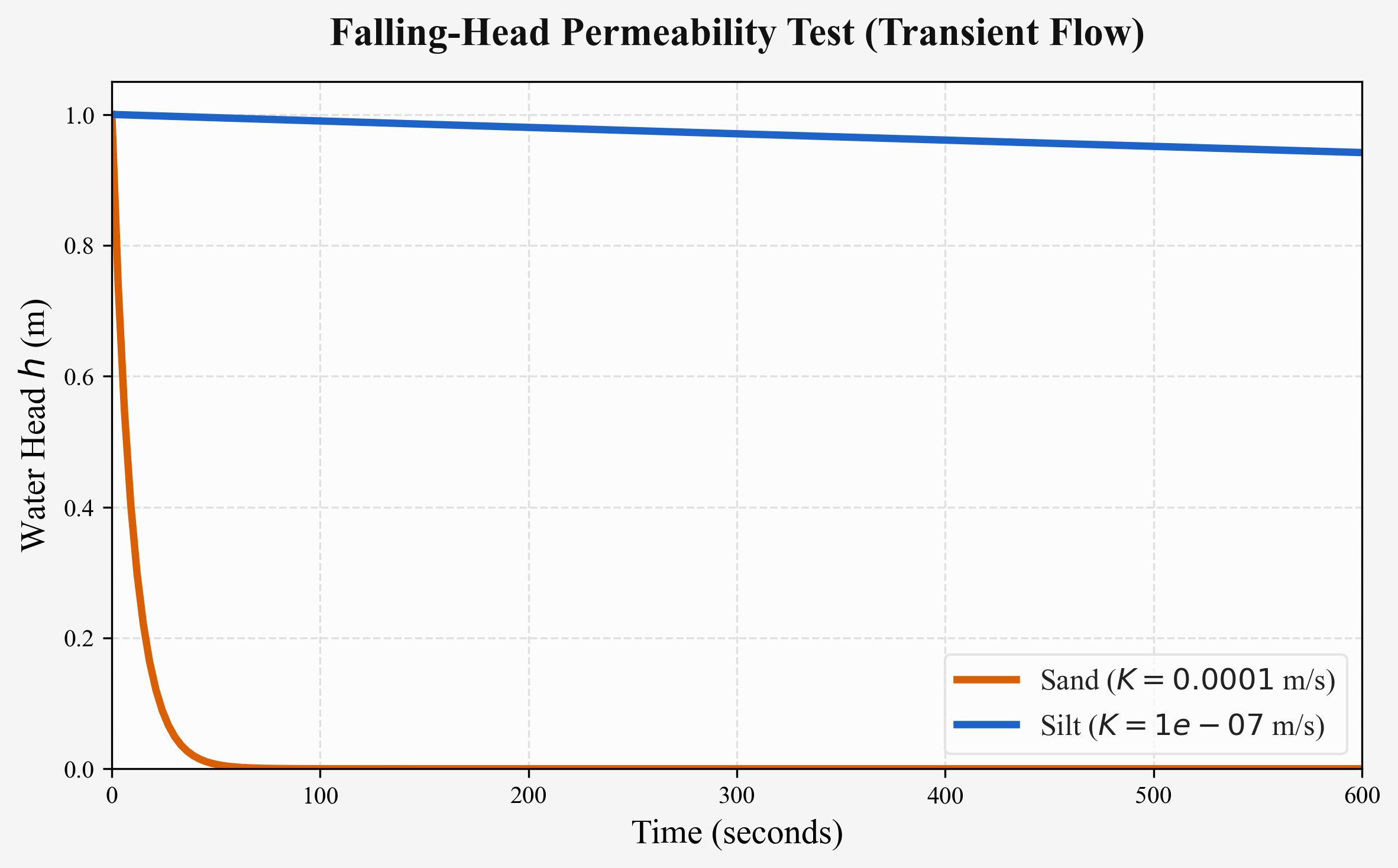
Because the orange “Sand” has high permeability, the water drains out quickly, and the water level approaches zero in no time. Meanwhile, the blue “Silt” sees its water level drop very gradually. This state of changing over time, drawing a curve, is exactly what transient flow looks like.
Show Python Code (Calculation and Simulation of Falling-Head Test)
import numpy as np
import matplotlib.pyplot as plt

# 1. Apparatus dimensions (defining variables)
r_pipe = 0.4      # Standpipe radius (cm)
r_sample = 2.5    # Sample radius (cm)

a = np.pi * r_pipe**2    # Standpipe area a (approx. 0.503 cm2)
A = np.pi * r_sample**2  # Sample area A (approx. 19.6 cm2)
L = 5.1                  # Sample length (cm)

h1 = 18.0                # Initial head (cm)
h2 = 8.0                 # Head after t seconds (cm)
t_meas = 360.0           # Measurement time (6 minutes = 360 seconds)

# 2. Formula for Saturated Hydraulic Conductivity
def calc_K(a, A, L, t, h1, h2):
    # K = (2.3 * a * L) / (A * t) * log10(h1 / h2)
    # (Note: 2.3 * log10 is an approximation for natural log ln)
    K = (2.3 * a * L) / (A * t) * np.log10(h1 / h2)
    return K

K_sample = calc_K(a, A, L, t_meas, h1, h2)
print(f"Calculated K: {K_sample:.2e} cm/sec")

# 3. Water viscosity and temperature correction (15°C)
def calc_viscosity(Wt):
    """Calculate water viscosity η at temperature Wt (°C)"""
    term1 = Wt - 8.435
    term2 = np.sqrt(8078.4 + term1**2)
    eta = 100 / (2.1482 * (term1 + term2) - 120)
    return eta

Wt_measure = 20.0  # Water temperature during measurement (e.g., 20°C)
eta_T = calc_viscosity(Wt_measure)
eta_15 = calc_viscosity(15.0)

K_15 = K_sample * (eta_T / eta_15)
print(f"Corrected K at 15°C: {K_15:.2e} cm/sec")

# 4. Simulation of falling head
# Calculate head change over time h(t) for a given K_sim
def simulate_falling_head(K_sim, t_array):
    alpha = (K_sim * A) / (a * L)
    # Analytical solution: h(t) = h1 * exp(-alpha * t)
    return h1 * np.exp(-alpha * t_array)

t_array = np.linspace(0, 600, 200) # 0 to 600 seconds
K_sand = 1e-3   # K for sand (cm/sec)
K_silt = 1e-5   # K for silt (cm/sec)

h_sand = simulate_falling_head(K_sand, t_array)
h_silt = simulate_falling_head(K_silt, t_array)

# (Plotting code omitted: plot t_array and h using matplotlib)
2.3 Why Aren’t Lab Tests Enough? (The Problem of Heterogeneity)
Lab tests are cheap and easy, but they can only measure a “point” data from a small, often disturbed soil sample of a few centimeters in diameter. Real geological formations are rarely perfectly homogeneous; they contain macro-scale Heterogeneity such as cracks, fractures, and complex interbedded layers of gravel lenses and clay. These tiny lab samples completely miss the impact of such large-scale features.
Therefore, to measure the average properties of the actual formation as an area (capturing realistic hydraulic properties including the scale effect), we take our tests out to the massive outdoor field—this is the Pumping Test. Only through this test can we obtain the two indispensable parameters for predictive simulation: the formation’s ability to transmit water (Transmissivity \(T\)) and its ability to store water (Storativity \(S\)).
3 Theory of Pumping Tests: Theis Equation
3.1 Inspiration from Heat Conduction
Before the 1930s, pumping test data were analyzed using equations that assumed the water level had perfectly stabilized (steady state). However, in reality, water levels rarely reach a perfect equilibrium during short-term tests.
C.V. Theis, a hydrologist at the USGS, struggled with this problem. One day, he realized that there is a deep physical and mathematical analogy between groundwater flow and heat conduction, and he wrote to his mathematician friend (Freeze and Cherry 1979).
“There is a close analogy between the flow of groundwater and the flow of heat. The quantities corresponding to the temperature gradient, thermal conductivity, and specific heat… Can a problem already solved in heat conduction approximate our problem?”
From this brilliant insight, Theis applied a known solution for heat conduction to groundwater, publishing the groundbreaking Theis Non-Equilibrium Equation in 1935 (Theis 1935).
3.2 Following the Math
When water is pumped at a constant rate from a fully confined, infinite aquifer, the drawdown \(s\) is described by the Theis equation:
\[ s = \frac{Q}{4 \pi T} W(u) \]
\[ u = \frac{r^2 S}{4 T t} \]
It looks a bit complicated, but let’s break it down piece by piece.
- \(s\) : How much the water level dropped (Drawdown) [m]
- \(Q\) : How much water the pump extracts (Pumping Rate) [m³/day]
- \(T\) : The aquifer’s ability to transmit water (Transmissivity) [m²/day]
- \(S\) : The aquifer’s ability to store water (Storativity) [-]
- \(r\) : Distance from the well to the observation point [m]
- \(t\) : Time elapsed since pumping started [day]
\(W(u)\) is a slightly special mathematical function (an exponential integral) called the Theis Well Function. The most important part is what’s inside \(u\).
\[u = \frac{\text{Distance } r^2 \times \text{Storage } S}{4 \times \text{Transmissivity } T \times \text{Time } t}\]
The value of \(u\) becomes larger when the distance \(r\) is large, or the time \(t\) is small. Conversely, as \(u\) gets smaller, \(W(u)\) gets larger, resulting in a larger drawdown \(s\). Intuitively, this perfectly matches our natural sense: the closer you are to the well, or the longer you keep pumping, the more the water level drops.
4 An Easier Way: Cooper-Jacob Straight-Line Method
While the Theis equation is powerful, calculating \(T\) and \(S\) backward by hand was incredibly tedious due to the special \(W(u)\) function.
In 1946, Cooper and Jacob discovered that if enough time has passed, and you are close enough to the well (specifically when \(u\) is less than 0.01), you can skip the complex function calculation and approximate it with a much simpler equation (Cooper and Jacob 1946). This is the Cooper-Jacob Method.
\[ s \approx \frac{2.303 Q}{4 \pi T} \log_{10} \left( \frac{2.25 T t}{r^2 S} \right) \]
The beauty of this equation is that the drawdown \(s\) becomes a linear function of the logarithm of time (\(\log_{10} t\)). This means if you plot the time on a logarithmic axis (scaling up like 1, 10, 100) and the drawdown on a regular vertical axis, the data points will line up perfectly straight.
4.1 Visualizing Pumping Tests with Python
Let’s use Python to see the “Cone of Depression” drawn by the Theis equation, and the “Straight Line” shown by Jacob’s law.
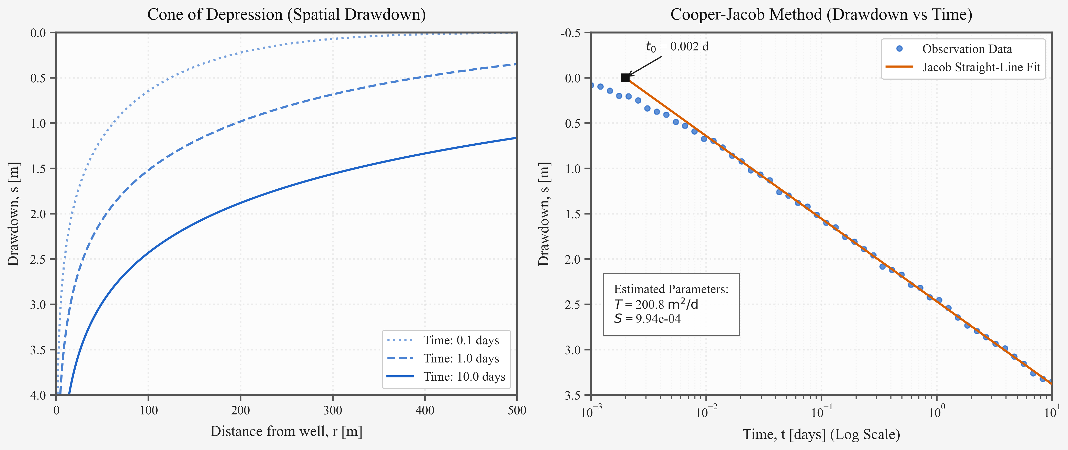
The left panel shows how the cone of depression deepens and widens over time—from 0.1 days, to 1 day, to 10 days after pumping begins.
The right panel plots the drawdown over time at an observation well 30 meters away. Notice how the horizontal axis is on a log scale. The data points to the right of the dashed line (after \(u < 0.01\) is satisfied) form a beautiful straight line. In practice, hydrogeologists calculate the transmissivity \(T\) from the “slope of this line,” and the storativity \(S\) from the “time it intersects the horizontal axis (\(t_0\)).”
Show Python Code (Theis function & Jacob method)
import numpy as np
import matplotlib.pyplot as plt
from scipy.special import exp1

# 1. Parameter Definition
Q = 1000.0   # Pumping rate (m3/day)
T = 200.0    # Transmissivity (m2/day)
S = 0.001    # Storativity (-)

def theis_drawdown(r, t, Q, T, S):
    """Calculate drawdown based on the Theis equation"""
    u = (r**2 * S) / (4.0 * T * t)
    # Scipy's exp1 corresponds to the Theis Well Function W(u)
    s = (Q / (4.0 * np.pi * T)) * exp1(u)
    return s

# 2. Jacob Method Analysis (Distance 30m)
r_obs = 30.0
t_times = np.logspace(-3, 1, 50)
s_time = theis_drawdown(r_obs, t_times, Q, T, S)

# Add noise to simulate real field data
np.random.seed(42)
s_noisy = s_time + np.random.normal(0, 0.02, size=len(s_time))

# Draw a line for data where u < 0.01
t_crit = (r_obs**2 * S) / (0.04 * T)
valid_idx = np.where(t_times > t_crit)[0]

if len(valid_idx) > 2:
    log_t_valid = np.log10(t_times[valid_idx])
    s_valid = s_noisy[valid_idx]
    coeffs = np.polyfit(log_t_valid, s_valid, 1) # Least squares fit

    # Extract T and S from the slope (delta_s)
    delta_s = coeffs[0]
    t0 = 10**(-coeffs[1] / coeffs[0]) # Time when s=0

    T_est = (2.303 * Q) / (4 * np.pi * delta_s)
    S_est = (2.25 * T_est * t0) / (r_obs**2)

    print(f"Results: T = {T_est:.1f} m2/d, S = {S_est:.2e}")
5 Modeling Wall: Peaceman’s Well Model
So far, we’ve looked at the beautiful mathematics of Theis. But when we try to simulate a well in a numerical grid simulation like MODFLOW, we hit a massive wall.
That wall is the “Scale Gap.”
A real well is only a few dozen centimeters in diameter. Meanwhile, a simulation grid cell is typically 10 to 100 meters across. The water level that MODFLOW calculates is “the average water level of that entire giant cell.” However, what we really want to know is “how deep the water level drops inside the narrow wellbore itself.” The two are definitely not the same.
5.1 The Idea of Equivalent Well Radius
D.W. Peaceman solved this problem in 1983 (Peaceman 1983). He mathematically proved the answer to the question: “At what radial distance \(r\) from the well does the analytical water level match the cell’s average water level?”
For a square cell (with sides of length \(\Delta x\)), he proved that the average cell head equals the head at a distance of \(r_e \approx 0.2 \Delta x\) from the well center. This \(r_e\) is called the Equivalent Well Radius.
Seeing is believing. I plotted this scale difference in Python.
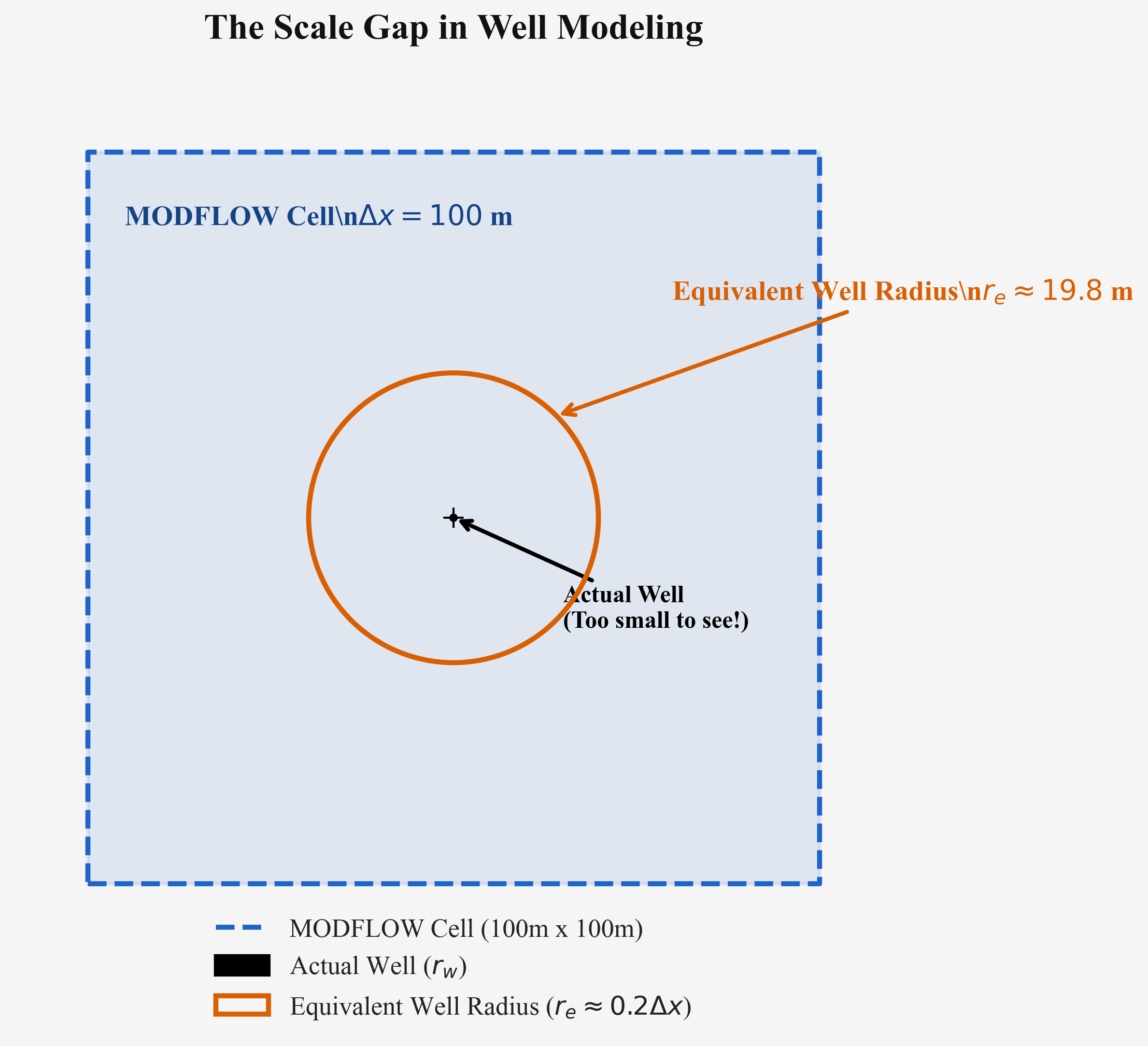
A real well is located in the center of the massive 100m x 100m MODFLOW cell (blue dashed line). However, the real well (about 15cm radius) is so small it just looks like a tiny black speck. Peaceman figured out that the average head of this entire MODFLOW cell corresponds to the head at the edge of the orange circle (a virtual well with a radius of about 20m).
Using this concept, the relationship between the cell’s average head \(h_{i,j}\) and the actual wellbore water level \(h_w\) is bridged by a coefficient called the Well Index (\(WI\)).
\[ Q = WI \times (h_{i,j} - h_w) \] \[ WI = \frac{2 \pi T}{\ln(r_e / r_w)} \]
When you use the WEL (Well) package in MODFLOW, Peaceman’s theory quietly works behind the scenes, bridging the immense “scale gap” between the giant grid and the tiny well.
Show Python Code (Plotting the Scale Gap)
import matplotlib.pyplot as plt
import matplotlib.patches as patches

# Cell size 100m
dx, dy = 100.0, 100.0
cx, cy = 0.0, 0.0

fig, ax = plt.subplots(figsize=(8, 8))

# MODFLOW Cell
rect = patches.Rectangle((cx - dx/2, cy - dy/2), dx, dy,
                         linewidth=2, edgecolor='#1E64C8', facecolor='#1E64C8', alpha=0.1)
ax.add_patch(rect)
ax.plot([cx - dx/2, cx + dx/2, cx + dx/2, cx - dx/2, cx - dx/2],
        [cy - dy/2, cy - dy/2, cy + dy/2, cy + dy/2, cy - dy/2],
        color='#1E64C8', lw=2.5, linestyle='--')

# Actual Well (Too small to see!)
well = patches.Circle((cx, cy), 0.3, linewidth=2, edgecolor='black', facecolor='black', zorder=5)
ax.add_patch(well)

# Peaceman's Equivalent Well Radius
r_e = 0.198 * dx
eq_well = patches.Circle((cx, cy), r_e, linewidth=2.5, edgecolor='#D95F02', facecolor='none', linestyle='-', zorder=4)
ax.add_patch(eq_well)

ax.set_aspect('equal')
ax.set_xlim(-60, 60)
ax.set_ylim(-60, 60)
ax.axis('off')
plt.title("The Scale Gap in Well Modeling", fontsize=16)
plt.show()
6 Conclusion
In this episode, we explored the world of transient flow, which changes over time, using pumping tests as our theme.
The Theis non-equilibrium equation is a monumental achievement in groundwater science, born from a beautiful analogy with heat conduction. With the Cooper-Jacob straight-line method, we can intuitively decipher the properties of geologic formations from field data. Finally, by learning about Peaceman’s well model, we saw just how cleverly our simulation software (MODFLOW) corrects the “discrepancies with reality” behind the scenes.
Next time, we will explore the places where groundwater emerges back to the surface—the relationship between rivers and groundwater. We’ll unravel the simple yet profound question: “Why doesn’t the river run dry when it hasn’t rained?”
7 References
8 Series List (Introduction to Groundwater Science)
- Part 1: What is the Water Cycle? — Where Does the Rain Go?
- Part 2: Where Does Groundwater Exist and How Does It Move? — Geological Vessels and Topographic Engines
- Part 3: Why Does Groundwater Move? — Darcy’s Law and the Physics of Head
- Part 4: Permeability & Pumping Tests and Well Modeling — How Do We Measure Aquifer Properties? (This article)
- Part 5: The Relationship Between Rivers and Groundwater (Forthcoming)