Introduction: Why Integrate with Python?
While PHREEQC’s built-in USER_GRAPH is handy for quick plots, Python is undeniably superior when it comes to creating publication-quality figures, interactive visualizations, and statistical processing. In this article, we will load the gibbsite_solubility.txt output from Part 7 into Python to achieve the following:
- You must have run the PHREEQC code from Part 7 and have the
gibbsite_solubility.txtfile ready. - You must have Python 3.9+ installed, along with
pandas,matplotlib,kaleidoandplotly.
(pip install pandas matplotlib kaleido plotly) kaleido is for exporting images from plotly. - pip is Python’s package management tool. You can install the required libraries by running the above command in a terminal (command prompt).
- Example:
pip install phreeqpyinstalls phreeqpy. The command above installs pandas, matplotlib, plotly, and kaleido all at once.
Step 1: Understanding the SELECTED_OUTPUT Structure
The file generated by PHREEQC’s SELECTED_OUTPUT is a tab-separated text file. The first line is the header, and the subsequent lines are the data.
# gibbsite_solubility.txt
sim state   soln    dist_x  pH  Al Al+3    AlOH+2  Al(OH)2+    Al(OH)3 Al(OH)4-    Gibbsite
1   i_soln  1   -1  7.000   0.000e+00   ...
2   react   1   -1  3.000   3.000   7.76e-03    -2.110  -5.270  -7.970  -9.710  -13.5   ...
3   react   2   -1  4.000   7.76e-04    -3.110  -5.270  -6.970  -9.710  -13.5   ...
...
Species specified via -activities are output in \(\log_{10}(\text{activity})\). Conversely, the Al specified via -totals is output in linear scale (mol/kgw). Before visualizing, you need to convert the total Al column to log scale while leaving the activity columns as they are.
Also, depending on your PHREEQC version, the header line might start directly with "pH Al..." instead of "sim state...".
Step 2: Loading Data with pandas
# ============================================================
#  phreeqc_read.py
#  Loading and cleaning PHREEQC SELECTED_OUTPUT files
# ============================================================
import pandas as pd
import numpy as np
from pathlib import Path

# ---- File Loading ----
fp = Path("gibbsite_solubility.txt")

df_raw = pd.read_csv(
    fp,
    sep="\t",             # Tab-separated
    comment="#",          # Skip comment lines
    skipinitialspace=True # Clean up whitespace
)

print(f"Shape: {df_raw.shape}")
print(df_raw.head())
print("\nColumns:", df_raw.columns.tolist())
> Columns: ['sim', 'state', 'soln', 'dist_x', 'pH', 'Al', 'la_Al+3',
'la_AlOH+2', 'la_Al(OH)2+', 'la_Al(OH)3', 'la_Al(OH)4-', 'Gibbsite']
# ---- Cleaning: Keep only the pH data rows ----
df = (
    df_raw
    # .query("state == 'react'")          # Optional: keep only equilibrium results
    .rename(columns={
        "Al":             "Al_total_mol",  # total Al (linear scale)
        "la_Al+3":        "log_Al3",
        "la_AlOH+2":      "log_AlOH2",
        "la_Al(OH)2+":    "log_AlOH2p",
        "la_Al(OH)3":     "log_AlOH3",
        "la_Al(OH)4-":    "log_AlOH4",
    })
    .reset_index(drop=True)
)

# ---- Convert total Al to log scale ----
df["log_Al_total"] = np.log10(df["Al_total_mol"].clip(lower=1e-15))

print(df[["pH", "log_Al_total", "log_Al3", "log_AlOH2p", "log_AlOH3","log_AlOH4"]].to_string(index=False))| pH | log_Al_total | log_Al3 | log_AlOH2p | log_AlOH3 | log_AlOH4 |
|---|---|---|---|---|---|
| 3.12 | 0.45 | -0.98 | -5.03 | -8.83 | -11.52 |
| 4.00 | -3.71 | -3.89 | -6.00 | -8.83 | -10.56 |
| 5.00 | -6.44 | -6.89 | -7.00 | -8.83 | -9.56 |
| 6.00 ★ | -7.80 | -9.89 | -8.00 | -8.83 | -8.56 |
| 7.00 | -7.52 | -12.89 | -9.00 | -8.83 | -7.56 |
| 8.00 | -6.55 | -15.89 | -10.00 | -8.83 | -6.56 |
| 9.00 | -5.55 | -18.89 | -11.00 | -8.83 | -5.56 |
| 10.00 | -4.55 | -21.89 | -12.00 | -8.83 | -4.56 |
Step 3: Plotting Publication-Quality Figures with matplotlib
Append the following code below Step 2 to generate the plot. Note that the plot labels have been localized to English for broad usability.
# ============================================================
#  phreeqc_plot_matplotlib.py
# ============================================================
import matplotlib.pyplot as plt
import matplotlib.ticker as ticker

# ---- Matplotlib Configuration ----
plt.rcParams.update({
    "font.family": "sans-serif",
    "axes.unicode_minus": False,
    "figure.dpi": 150,
})

# ---- Data Preparation ----
ph = df["pH"].values

species = {
    "Total Al":      ("log_Al_total", "#111827", 2.8, "-",  "o"),
    r"Al$^{3+}$":    ("log_Al3",      "#DC2626", 1.8, "-",  "s"),
    r"AlOH$^{2+}$":  ("log_AlOH2",   "#EA580C", 1.6, "--", "^"),
    r"Al(OH)$_2^+$": ("log_AlOH2p",  "#CA8A04", 1.6, "-.", "D"),
    r"Al(OH)$_3$(aq)":("log_AlOH3",  "#16A34A", 1.6, ":",  ""),
    r"Al(OH)$_4^-$": ("log_AlOH4",   "#2563EB", 1.8, "-",  "v"),
}

fig, ax = plt.subplots(figsize=(9, 6))

# ---- Gibbsite Stability Background ----
ax.axvspan(5.5, 8.5, alpha=0.07, color="#16A34A", label="_nolegend_")
ax.text(7.0, -2.3, "Gibbsite\nStability Zone", ha="center", va="top",
        fontsize=10, color="#15803D", style="italic")

# ---- Plot Each Species ----
for label, (col, color, lw, ls, marker) in species.items():
    y = df[col].replace([np.inf, -np.inf], np.nan).values
    valid = ~np.isnan(y) & (y > -12)          # Only plot values above detection limit
    if marker:
        ax.plot(ph[valid], y[valid], color=color, lw=lw,
                ls=ls, marker=marker, ms=5, label=label)
    else:
        ax.plot(ph[valid], y[valid], color=color, lw=lw,
                ls=ls, label=label)

# ---- Minimum Value Annotation ----
min_idx = df["log_Al_total"].idxmin()
min_ph  = df.loc[min_idx, "pH"]
min_log = df.loc[min_idx, "log_Al_total"]
ax.annotate(
    f"Minimum\npH ≈ {min_ph:.1f}\n10⁻⁷ mol/L",
    xy=(min_ph, min_log),
    xytext=(min_ph + 1.5, min_log + 1.2),
    fontsize=9, color="#92400E",
    arrowprops=dict(arrowstyle="->", color="#D97706", lw=1.5),
    bbox=dict(boxstyle="round,pad=0.3", fc="#FEF3C7", ec="#D97706", alpha=0.9),
)

# ---- Axes and Formatting ----
ax.set_xlim(3, 14)
ax.set_ylim(-11, 0.5)
ax.set_xlabel("pH", fontsize=13)
ax.set_ylabel(r"$\log$ [Al]  (mol/kgw)", fontsize=13)
ax.set_title("Gibbsite Solubility Diagram (Al–H₂O System, 25°C)", fontsize=14, pad=12)
ax.xaxis.set_major_locator(ticker.MultipleLocator(1))
ax.yaxis.set_major_locator(ticker.MultipleLocator(1))
ax.grid(True, which="major", ls="--", lw=0.5, color="#E5E7EB")
ax.legend(loc="upper right", fontsize=10, framealpha=0.95)

plt.tight_layout()
plt.savefig("gibbsite_solubility.png", dpi=300, bbox_inches="tight")
plt.savefig("gibbsite_solubility.svg", bbox_inches="tight")   # Vector format
plt.show()
print("✅ Saved successfully: gibbsite_solubility.png / .svg")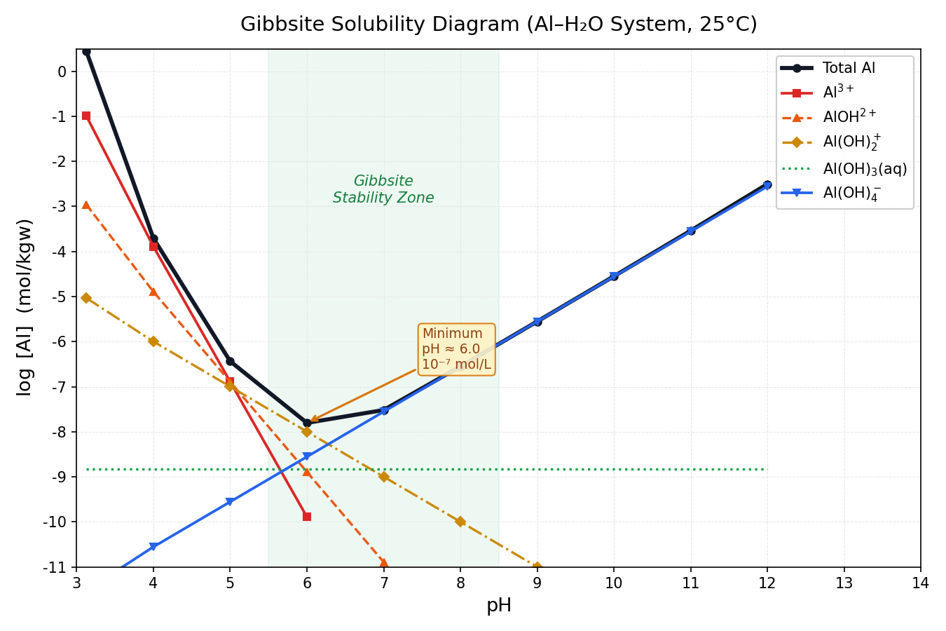
Step 4: Dominant Species Map (Speciation Diagram)
In geochemistry, it is equally important to visualize which species is dominant at a given pH.
# ============================================================
#  phreeqc_speciation_map.py
#  Mapping dominant Al species by color across pH
# ============================================================
import matplotlib.patches as mpatches

# Determine the maximum activity species at each pH
activity_cols = ["log_Al3", "log_AlOH2", "log_AlOH2p", "log_AlOH3", "log_AlOH4"]
species_names  = ["Al³⁺", "AlOH²⁺", "Al(OH)₂⁺", "Al(OH)₃(aq)", "Al(OH)₄⁻"]
species_colors = ["#DC2626", "#EA580C", "#CA8A04", "#16A34A", "#2563EB"]

df_act = df[activity_cols].replace([np.inf, -np.inf], np.nan).fillna(-99)
dominant_idx = df_act.values.argmax(axis=1)

fig, ax = plt.subplots(figsize=(10, 2.2))

for i, row in df.iterrows():
    ph_val = row["pH"]
    d_idx  = dominant_idx[i]
    color  = species_colors[d_idx]
    rect   = mpatches.FancyBboxPatch(
        (ph_val - 0.45, 0.1), 0.9, 0.8,
        boxstyle="round,pad=0.05",
        facecolor=color, edgecolor="white", linewidth=1.5, alpha=0.85,
    )
    ax.add_patch(rect)
    ax.text(ph_val, 0.5, species_names[d_idx],
            ha="center", va="center", fontsize=8, color="white", fontweight="bold")

ax.set_xlim(2.5, 12.5)
ax.set_ylim(0, 1)
ax.set_xlabel("pH", fontsize=12)
ax.set_yticks([])
ax.set_xticks(range(3, 13))
ax.set_title("Al Dominant Species Map (Gibbsite Equilibrium, 25°C)", fontsize=12, pad=8)

# Legend
patches = [mpatches.Patch(color=c, label=n)
           for c, n in zip(species_colors, species_names)]
ax.legend(handles=patches, loc="upper center",
          bbox_to_anchor=(0.5, -0.35), ncol=5, fontsize=9, framealpha=0.9)

plt.tight_layout()
plt.savefig("al_speciation_map.svg", bbox_inches="tight")
plt.show()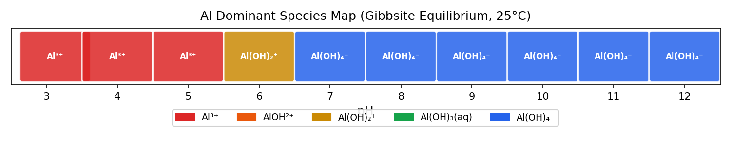
Step 5: The Complete Analytical Workflow (One-File Script)
Below is the complete, consolidated script covering Steps 1 through 4. Simply copy, paste, and run this code alongside your gibbsite_solubility.txt.
#  gibbsite_full_analysis.py
#  Complete Analysis Script for PHREEQC Part 7
#  Usage: python gibbsite_full_analysis.py gibbsite_solubility.txt
# ============================================================
import sys
import numpy as np
import pandas as pd
import matplotlib.pyplot as plt
import matplotlib.ticker as ticker
import matplotlib.patches as mpatches

plt.rcParams.update({
    "font.family": "sans-serif",
    "axes.unicode_minus": False,
    "figure.dpi": 150,
})

# ---- Constants ----
SPECIES = {
    "Total Al":       ("log_Al_total", "#111827", 2.8, "-"),
    r"Al$^{3+}$":     ("log_Al3",      "#DC2626", 1.8, "-"),
    r"AlOH$^{2+}$":   ("log_AlOH2",   "#EA580C", 1.6, "--"),
    r"Al(OH)$_2^+$":  ("log_AlOH2p",  "#CA8A04", 1.6, "-."),
    r"Al(OH)$_3$":    ("log_AlOH3",   "#16A34A", 1.6, ":"),
    r"Al(OH)$_4^-$":  ("log_AlOH4",   "#2563EB", 1.8, "-"),
}

ACT_COLS  = ["log_Al3", "log_AlOH2", "log_AlOH2p", "log_AlOH3", "log_AlOH4"]
SP_NAMES  = [r"Al$^{3+}$", r"AlOH$^{2+}$", r"Al(OH)$_2^+$",
             r"Al(OH)$_3$(aq)", r"Al(OH)$_4^-$"]
SP_COLORS = ["#DC2626", "#EA580C", "#CA8A04", "#16A34A", "#2563EB"]

def load_data(filepath: str) -> pd.DataFrame:
    """Load and format SELECTED_OUTPUT."""
    df = pd.read_csv(filepath, sep="\t", comment="#", skipinitialspace=True)
    df = df.rename(columns={
        "Al": "Al_total_mol",
        "la_Al+3": "log_Al3", "la_AlOH+2": "log_AlOH2",
        "la_Al(OH)2+": "log_AlOH2p", "la_Al(OH)3": "log_AlOH3", "la_Al(OH)4-": "log_AlOH4",
    })
    df["log_Al_total"] = np.log10(df["Al_total_mol"].clip(lower=1e-15))
    return df

def plot_solubility(df: pd.DataFrame, save: bool = True):
    """Render the Solubility Diagram."""
    fig, ax = plt.subplots(figsize=(9, 6))
    ax.axvspan(5.5, 8.5, alpha=0.07, color="#16A34A")
    ax.text(7.0, -2.0, "Gibbsite\nStability Zone", ha="center",
            fontsize=10, color="#15803D", style="italic")

    for label, (col, color, lw, ls) in SPECIES.items():
        y = df[col].replace([np.inf, -np.inf], np.nan).values
        mask = ~np.isnan(y) & (y > -12)
        ax.plot(df["pH"].values[mask], y[mask],
                color=color, lw=lw, ls=ls, label=label, marker="o", ms=4)

    mi = df["log_Al_total"].idxmin()
    ax.annotate(
        f"Min pH ≈ {df.loc[mi,'pH']:.1f}",
        xy=(df.loc[mi, "pH"], df.loc[mi, "log_Al_total"]),
        xytext=(df.loc[mi, "pH"] + 1.5, df.loc[mi, "log_Al_total"] + 1.5),
        fontsize=9, color="#92400E",
        arrowprops=dict(arrowstyle="->", color="#D97706"),
        bbox=dict(boxstyle="round", fc="#FEF3C7", ec="#D97706"),
    )

    ax.set(xlim=(3, 14), ylim=(-11, 0.5),
           xlabel="pH", ylabel=r"$\log$ [Al] (mol/kgw)",
           title="Gibbsite Solubility Diagram (Al–H₂O System, 25°C)")
    ax.xaxis.set_major_locator(ticker.MultipleLocator(1))
    ax.yaxis.set_major_locator(ticker.MultipleLocator(1))
    ax.grid(True, ls="--", lw=0.5, color="#E5E7EB")
    ax.legend(fontsize=10, loc="upper right")
    plt.tight_layout()
    if save:
        fig.savefig("gibbsite_solubility.svg", bbox_inches="tight")
        print("✅ Saved gibbsite_solubility.svg")
    plt.show()

def plot_speciation_map(df: pd.DataFrame, save: bool = True):
    """Render the Dominant Species Map."""
    df_act = df[ACT_COLS].replace([np.inf, -np.inf], np.nan).fillna(-99)
    dom = df_act.values.argmax(axis=1)

    fig, ax = plt.subplots(figsize=(10, 2.2))
    for i, row in df.iterrows():
        c = SP_COLORS[dom[i]]
        rect = mpatches.FancyBboxPatch(
            (row["pH"] - 0.45, 0.1), 0.9, 0.8,
            boxstyle="round,pad=0.05",
            facecolor=c, edgecolor="white", lw=1.5, alpha=0.85,
        )
        ax.add_patch(rect)
        ax.text(row["pH"], 0.5, SP_NAMES[dom[i]],
                ha="center", va="center", fontsize=8,
                color="white", fontweight="bold")

    patches = [mpatches.Patch(color=c, label=n)
               for c, n in zip(SP_COLORS, SP_NAMES)]
    ax.set(xlim=(2.5, 12.5), ylim=(0, 1),
           xlabel="pH", title="Al Dominant Species Map (Gibbsite Eq, 25°C)")
    ax.set_yticks([])
    ax.set_xticks(range(3, 13))
    ax.legend(handles=patches, loc="upper center",
              bbox_to_anchor=(0.5, -0.35), ncol=5, fontsize=9)
    plt.tight_layout()
    if save:
        fig.savefig("al_speciation_map.svg", bbox_inches="tight")
        print("✅ Saved al_speciation_map.svg")
    plt.show()

# ---- Main ----
if __name__ == "__main__":
    fp = sys.argv[1] if len(sys.argv) > 1 else "gibbsite_solubility.txt"
    df = load_data(fp)
    print(df[["pH", "log_Al_total", "log_Al3", "log_AlOH4"]].to_string(index=False))
    plot_solubility(df)
    plot_speciation_map(df)
Run with a single line:
python gibbsite_full_analysis.py gibbsite_solubility.txtSummary: The PHREEQC × Python Workflow
→ Output TXT
→ Load to pandas
Automate in a single script
Next time, in Part 9, we will dive into Ionic Strength and Activity Coefficients—the reasons why calculation results differ between seawater and freshwater.
References
- #1 Installation and Initial Calculation
- #2 Analyzing Seawater with Speciation
- #3 Mineral Equilibrium and Temperature Effects
- #4 Calcite–CO₂ Interaction (Open vs. Closed Systems)
- #5 Mixing Groundwater and Seawater
- #6 Pyrite Oxidation and AMD Formation
- #7 Solubility Diagrams (Gibbsite)
- #8 Visualization with Python (This article)
- #9 Ionic Strength and Activity Coefficients