Introduction: The “Unsolved Mystery” Since Part 2
From analyzing seawater speciation in Part 2 to calculating Gibbsite solubility in Part 7, a single underlying question has likely lingered in your mind throughout these calculations:
“Why do seawater and freshwater yield different calculation results even when the pH and temperature are identical?”
The answer lies in Activity. PHREEQC does not use concentration (mol/kgw) directly to calculate chemical equilibrium; instead, it uses activity, which is concentration multiplied by a “correction factor.” This correction factor is known as the activity coefficient, \(\gamma\) (gamma).
γi: Activity coefficient (0 < γ ≤ 1)
mi: Molality (mol/kgw)
In dilute solutions, \(\gamma \approx 1\), meaning activity \(\approx\) concentration. However, in seawater (which has an ionic strength \(I \approx 0.7\) mol/kgw), \(\gamma\) drops below \(0.1\) for certain species. This creates an error that cannot be ignored.
- The definition and calculation of Ionic Strength (\(I\))
- The mechanics and applications of the four activity models: Debye-Hückel, Extended Debye-Hückel, Davies, and Pitzer
- How to configure activity coefficient models in PHREEQC (
-activity_coefficients) - Python code to compare results across the four models for the same solution
- A decision flow for choosing the right model
Theory Part 1: What is Ionic Strength?
Definition
Ionic strength (\(I\)) is a measure of the “charge-weighted concentration” of all ions in a solution:
\[I = \frac{1}{2} \sum_i m_i z_i^2\]
Where \(m_i\) is the molality of ion \(i\) (mol/kgw), and \(z_i\) is the valence (charge) of ion \(i\).
| Water Type | Composition | I (mol/kg) | Applicable Model |
|---|---|---|---|
| Distilled / Rainwater | Nearly pure water | < 0.001 | Debye-Hückel |
| River / Groundwater | Ca²⁺, HCO₃⁻ dominant | 0.001–0.05 | Extended Debye-Hückel |
| Brackish / Hot Springs | Increased Na⁺, Cl⁻ | 0.05–0.5 | Davies |
| Seawater | NaCl ≈ 0.5 M | ≈ 0.7 | Davies / Pitzer |
| Salt Lakes / Brines | Hyper-saline | > 1 | Pitzer required |
Hand-Calculating the Ionic Strength of Seawater
Na⁺ = 0.4689, z = +1 → 0.4689 × 1² = 0.4689
Cl⁻ = 0.5453, z = −1 → 0.5453 × 1² = 0.5453
Mg²⁺ = 0.0528, z = +2 → 0.0528 × 4 = 0.2112
SO₄²⁻= 0.0283, z = −2 → 0.0283 × 4 = 0.1132
Ca²⁺ = 0.0103, z = +2 → 0.0103 × 4 = 0.0412
K⁺ = 0.0102, z = +1 → 0.0102 × 1 = 0.0102
──────────────────────────────────────
Sum = 1.3900
I = 1.3900 / 2 = 0.695 mol/kg
Theory Part 2: The Four Activity Coefficient Models
Model 1: Debye-Hückel (DH)
The simplest theoretical equation, considering only the Coulombic attraction between ions:
\[\log \gamma_i = -A z_i^2 \sqrt{I}\]
\(A = 0.509\) (for water at 25°C). This is valid only for extremely dilute solutions where \(I < 0.005\) mol/kg.
Model 2: Extended Debye-Hückel (LLNL form)
An improved version that incorporates the effective ionic radius (\(a_i\)):
\[\log \gamma_i = \frac{-A z_i^2 \sqrt{I}}{1 + B a_i \sqrt{I}}\]
Where \(a_i\) is the effective radius (in Å) and \(B = 0.328\). Valid for \(I < 0.1\) mol/kg. This model is used by the standard PHREEQC databases (phreeqc.dat, llnl.dat).
Model 3: Davies
Adds an empirical correction term for higher ionic strengths:
\[\log \gamma_i = -A z_i^2 \left( \frac{\sqrt{I}}{1 + \sqrt{I}} - 0.3 I \right)\]
Valid up to \(I < 0.5\) mol/kg. It is highly suitable for brackish waters and soil waters. In PHREEQC, you can manually specify it using -activity_model davies.
Model 4: Pitzer
A highly accurate model using empirically derived interaction parameters (\(\beta^{(0)}\), \(\beta^{(1)}\), \(C^{\phi}\)) for specific ion pairs:
\[\ln \gamma_{\pm} = f(I) + \sum_{ij} B_{ij}(I) m_j + \sum_{ijk} C_{ijk} m_j m_k + \cdots\]
Mandatory for brines, salt lakes, and geothermal fluids where \(I > 0.5\) mol/kg. In PHREEQC, you must load the pitzer.dat database to use this model.
Comparing the Four Models with Python
The code below performs calculations using phreeqc.dat and llnl.dat.
However, an error occurs with phreeqc.dat when using Phreeqc Interactive 3.8.6-17100. Therefore, it is recommended to use wateq4f.dat or the newly added PHREEQC_ThermoddemV1.10_15Dec2020.dat instead. (Note that this issue does not occur in Phreeqc Interactive 3.7.3-15968.)
The following code assumes the use of Phreeqc Interactive 3.8.6-17100 and utilizes wateq4f.dat. Please pay close attention to the database file paths on your system.
For example, if llnl.dat is located in a folder named Phreeqc on your Desktop, the path would be specified as follows:
r"C:\Users\Desktop\Phreeqc\llnl.dat"
Please modify the file paths for DB_PHREEQC and DB_LLNL in the code below accordingly.
import os
import numpy as np
import pandas as pd
import matplotlib.pyplot as plt
from phreeqpy.iphreeqc.phreeqc_dll import IPhreeqc

# ==============================
# 1. Database Paths Configuration
# ==============================
# ***Please modify these to match your local paths***
DB_PHREEQC = r"C:\...\wateq4f.dat"
DB_LLNL    = r"C:\...\llnl.dat"

# ==============================
# 2. PHREEQC Input String
# ==============================
# We add 1.1 moles to ensure ionic strength exceeds 1.0
input_string = """
SOLUTION 1 Pure water
    temp 25
    pH 7 charge

REACTION 1
    NaCl 1.1
    1.1 moles in 100 steps

SELECTED_OUTPUT
    -reset false
    -user_punch true

USER_PUNCH
    -headings I Gamma_Na
    -start
    10 PUNCH MU, GAMMA("Na+")
    -end
"""

# ==============================
# 3. PHREEQC Execution Function
# ==============================
def run_phreeqc(db_path, label):
    db_path = os.path.abspath(db_path)
    print(f"Loading DB: {os.path.basename(db_path)} ...", end=" ")

    if not os.path.exists(db_path):
        raise FileNotFoundError(f"\n❌ Database not found: {db_path}")

    ip = IPhreeqc()

    try:
        ip.load_database(db_path)
    except Exception as e:
        raise RuntimeError(f"\n❌ Python Exception during load_database: {e}")

    error_str = ip.get_error_string()
    if error_str:
        raise RuntimeError(f"\n❌ Failed to load {label} DB (DLL Error):\n{error_str}")

    print("OK")

    try:
        ip.run_string(input_string)
    except Exception as e:
        error_str = ip.get_error_string()
        raise RuntimeError(f"\n❌ PHREEQC execution error for {label}:\n{e}\n{error_str}")

    out = ip.get_selected_output_array()

    if len(out) > 1:
        df = pd.DataFrame(out[1:], columns=out[0]).astype(float)
        return df
    return pd.DataFrame()

# ==============================
# 4. Theoretical Calculations
# ==============================
def calc_theoretical(I):
    A = 0.509
    z = 1.0

    gamma_dh = 10 ** (-A * (z**2) * np.sqrt(I))
    gamma_davies = 10 ** (-A * (z**2) * (np.sqrt(I) / (1 + np.sqrt(I)) - 0.3 * I))

    return gamma_dh, gamma_davies

# ==============================
# 5. Execution and Data Collection
# ==============================
if __name__ == "__main__":
    try:
        df_phreeqc = run_phreeqc(DB_PHREEQC, "PHREEQC")
        df_llnl    = run_phreeqc(DB_LLNL, "LLNL")

        # Exclude Step 0 (pure water) where gamma output might be 0
        df_phreeqc = df_phreeqc[df_phreeqc['Gamma_Na'] > 0]
        df_llnl    = df_llnl[df_llnl['Gamma_Na'] > 0]

        I_theory = np.linspace(0.001, 1.0, 100)
        gamma_dh, gamma_davies = calc_theoretical(I_theory)

        # ==============================
        # 6. Plotting
        # ==============================
        plt.rcParams['font.family'] = 'sans-serif'
        plt.rcParams['axes.unicode_minus'] = False

        fig, ax = plt.subplots(figsize=(8, 5))
        ax.set_facecolor('#F9FAFB')
        ax.grid(color='#E5E7EB', linestyle='-', linewidth=0.8)
        for spine in ax.spines.values():
            spine.set_color('#9CA3AF')

        ax.axhline(1.0, color='#D97706', linestyle='--', alpha=0.5, label='_nolegend_')
        ax.axvline(0.7, color='#DC2626', linestyle='--', alpha=0.5, label='_nolegend_')
        ax.text(0.71, 0.95, 'Seawater I ≈ 0.7', color='#DC2626', style='italic', fontsize=10)

        # Plot Data
        ax.plot(I_theory, gamma_dh, color='#6B7280', linestyle=':', linewidth=2, label='Debye-Hückel (Theoretical)')
        ax.plot(I_theory, gamma_davies, color='#16A34A', linestyle='--', linewidth=2, label='Davies (Theoretical)')
        ax.plot(df_phreeqc['I'], df_phreeqc['Gamma_Na'], color='#2563EB', linestyle='-', linewidth=2, label='WATEQ Eq (Extended D-H (wateq4f.dat))')
        ax.plot(df_llnl['I'], df_llnl['Gamma_Na'], color='#CA8A04', linestyle='-', linewidth=2, label='B-dot Eq (llnl.dat)')

        ax.set_xlabel('Ionic Strength I (mol/kgw)', fontsize=12, color='#374151')
        ax.set_ylabel(r'Activity Coefficient $\gamma$ (Na$^+$, z=1)', fontsize=12, color='#374151')

        ax.set_xlim(0, 1.0)
        ax.set_ylim(0, 1.05)
        ax.tick_params(colors='#6B7280')

        ax.legend(loc='lower right', facecolor='white', framealpha=0.9, edgecolor='#E5E7EB', fontsize=10)
        plt.title('Comparison of Activity Coefficient Models (25°C, Na⁺)', color='#374151', pad=15)

        plt.tight_layout()
        plt.savefig('Activity_Coefficients.png', dpi=300)
        plt.savefig('Activity_Coefficients.svg', bbox_inches='tight')
        plt.show()

        print("\n✅ Saved as 'Activity_Coefficients.png / .svg'")

    except Exception as e:
        print(f"\n🚨 Error occurred during execution:\n{e}")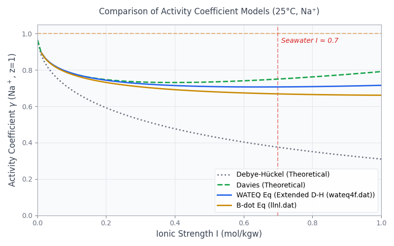
As ionic strength increases, the divergence between the activity coefficient models becomes significant.
Verifying Activity Coefficients in PHREEQC
You can back-calculate the exact \(\gamma\) values from SELECTED_OUTPUT using -activities and -totals:
# Checking Activity Coefficients
SOLUTION 1
    temp  25
    pH    8.22
    units mol/kgw
    Na    0.4689
    Cl    0.5453
    Mg    0.0528
    Ca    0.0103
    K     0.0102
    Alkalinity 2.3e-3 as HCO3
    S(6)  0.0283

SELECTED_OUTPUT 1
    -file     activity_check.txt
    -totals   Na Ca Mg Cl S(6) C(4)
    -activities Na+ Ca+2 Mg+2 Cl- SO4-2 HCO3-

USER_PUNCH 1
    -headings  Species  Molality  Activity  Gamma
    -start
    10 PUNCH "Na+",  MOL("Na+"),  ACT("Na+"),  ACT("Na+") /MOL("Na+")
    20 PUNCH "Ca+2", MOL("Ca+2"), ACT("Ca+2"), ACT("Ca+2")/MOL("Ca+2")
    30 PUNCH "Mg+2", MOL("Mg+2"), ACT("Mg+2"), ACT("Mg+2")/MOL("Mg+2")
    40 PUNCH "Cl-",  MOL("Cl-"),  ACT("Cl-"),  ACT("Cl-") /MOL("Cl-")
    50 PUNCH "SO4-2",MOL("SO4-2"),ACT("SO4-2"),ACT("SO4-2")/MOL("SO4-2")
END
Interpreting the Results
| Species | Valence z | Molality m | Activity a | Gamma γ | Meaning |
|---|---|---|---|---|---|
| Na⁺ | ±1 | 0.4689 | 0.361 | 0.77 | Activity is 77% of concentration. |
| Ca²⁺ | ±2 | 0.0103 | 0.00284 | 0.28 | Activity is only 28% of conc! |
| Mg²⁺ | ±2 | 0.0528 | 0.0148 | 0.28 | Divalent ions are suppressed heavily. |
| SO₄²⁻ | ±2 | 0.0283 | 0.0071 | 0.25 | Only effectively "acts" as 1/4th. |
Because the Debye-Hückel equation contains \(z^2\), a divalent ion is suppressed by a factor of 4 compared to a monovalent ion. It may seem counterintuitive that sulfate in seawater behaves as if only 1/4th of it is present, but this is exactly why neglecting activity leads to massive errors. The solubility product of Calcite (\(K_{sp}\)) is defined as \(a_{\mathrm{Ca^{2+}}} \cdot a_{\mathrm{CO_3^{2-}}}\). Evaluating it strictly by concentration leads to fundamentally flawed thermodynamic interpretations.
Visualizing Activity vs. Ionic Strength in Python
# ============================================================
#  activity_coeff_plot.py
# ============================================================
import numpy as np
import matplotlib.pyplot as plt

plt.rcParams.update({
    "font.family": "sans-serif",
    "axes.unicode_minus": False,
    "figure.dpi": 150,
})

# ---- Debye-Hückel Parameters (25°C, Water) ----
A = 0.509
B = 0.328e8 # Careful with units

# ---- Calculating Gamma across Models ----
I = np.linspace(0, 1.0, 500)

def gamma_dh(I, z=1):
    """Simple Debye-Hückel"""
    return 10 ** (-A * z**2 * np.sqrt(I))

def gamma_edh(I, z=1, a_param=4.0):
    """Extended Debye-Hückel"""
    B_prime = 0.328
    return 10 ** (-A * z**2 * np.sqrt(I) / (1 + B_prime * a_param * np.sqrt(I)))

def gamma_davies(I, z=1):
    """Davies Model"""
    return 10 ** (-A * z**2 * (np.sqrt(I)/(1+np.sqrt(I)) - 0.3*I))

def gamma_pitzer_approx(I, z=1):
    """Pitzer Approximation (fitted to NaCl empirical data)"""
    if z == 1:
        return 10 ** (-0.509 * np.sqrt(I) / (1 + 1.316 * np.sqrt(I)) + 0.09 * I)
    else:
        return 10 ** (-0.509 * z**2 * np.sqrt(I) / (1 + 1.316 * np.sqrt(I)) + 0.09 * I * z**2 * 0.3)

fig, axes = plt.subplots(1, 2, figsize=(12, 5))

# ---- Left: Comparing Models for z=1 ----
ax = axes[0]
ax.plot(I, gamma_dh(I, 1),          color="#6B7280", lw=1.8, ls="--", label="Debye-Hückel")
ax.plot(I, gamma_edh(I, 1),         color="#CA8A04", lw=2.0,          label="Extended D-H (a=4Å)")
ax.plot(I, gamma_davies(I, 1),      color="#16A34A", lw=2.0, ls="-.", label="Davies")
ax.plot(I, gamma_pitzer_approx(I,1),color="#2563EB", lw=2.5,          label="Pitzer (Approx)")
ax.axvline(0.7, color="#DC2626", lw=1, ls=":", alpha=0.7)
ax.text(0.72, 0.95, "Seawater\nI≈0.7", color="#DC2626", fontsize=9)
ax.set(xlim=(0,1), ylim=(0,1.05), xlabel="Ionic Strength I (mol/kg)",
       ylabel=r"$\gamma$", title="Models for Monovalent Ions (z = ±1)")
ax.legend(fontsize=9); ax.grid(True, ls="--", lw=0.5, color="#E5E7EB")

# ---- Right: Comparing Valences (Extended DH) ----
ax = axes[1]
for z, color, label in [(1,"#16A34A","z = ±1 (Na⁺, Cl⁻)"),
                         (2,"#EA580C","z = ±2 (Ca²⁺, SO₄²⁻)"),
                         (3,"#DC2626","z = ±3 (Al³⁺, PO₄³⁻)")]:
    ax.plot(I, gamma_edh(I, z), color=color, lw=2.2, label=label)
ax.axvline(0.7, color="#9CA3AF", lw=1, ls=":", alpha=0.7)
ax.set(xlim=(0,1), ylim=(0,1.05), xlabel="Ionic Strength I (mol/kg)",
       ylabel=r"$\gamma$", title="Effect of Valence (Extended D-H)")
ax.legend(fontsize=9); ax.grid(True, ls="--", lw=0.5, color="#E5E7EB")

plt.suptitle("Dependence of Activity Coefficient γ on Ionic Strength (25°C)", fontsize=13, y=1.02)
plt.tight_layout()
plt.savefig("activity_coefficient.svg", bbox_inches="tight")
plt.show()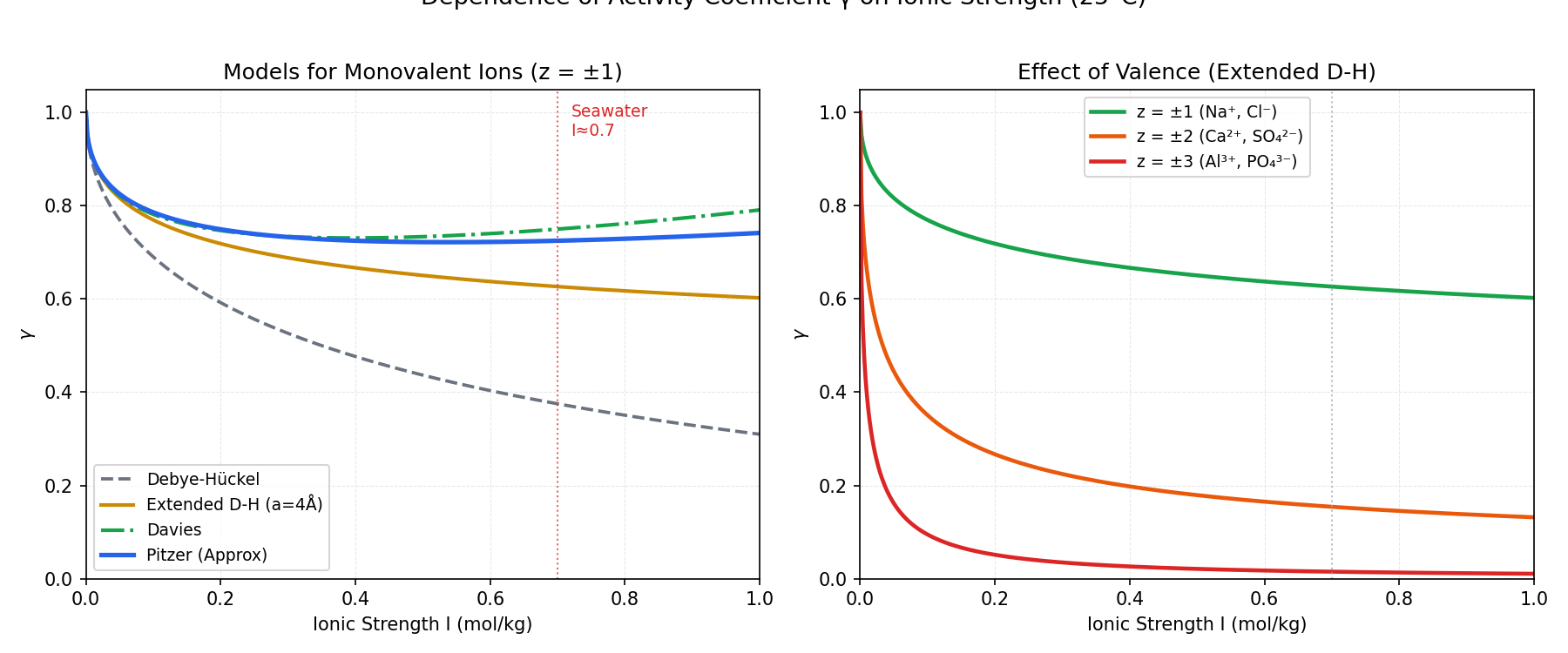
Summary: The Importance of Recognizing “Activity”
With a solid understanding of how to correctly compute activity, we can properly interpret the Saturation Index: \(SI = \log(IAP/K_{sp})\) for various minerals. If \(SI > 0\), precipitation occurs; if \(SI < 0\), dissolution happens. It turns out that every calculation we made from Part 2 to Part 7 was secretly relying on this exact logic!
By completing this article, the persistent “why?” that has been building up since Part 2 should finally be resolved. Knowing that PHREEQC automatically handles these complex corrections under the hood will entirely change how you read your simulation results.
References
- #1 Installation and Initial Calculation
- #2 Analyzing Seawater with Speciation
- #3 Mineral Equilibrium and Temperature Effects
- #4 Calcite–CO₂ Interaction (Open vs. Closed Systems)
- #5 Mixing Groundwater and Seawater
- #6 Pyrite Oxidation and AMD Formation
- #7 Solubility Diagrams (Gibbsite)
- #8 Visualization with Python
- #9 Ionic Strength and Activity Coefficients (This article)
- #10 Mastering the Saturation Index (SI)