Introduction to Groundwater Science #5: Where Does the River Water Come From? — Interaction Between River and Groundwater

1 Introduction: The Mystery of Persistent River Flow

Why do rivers continue to flow even when it hasn’t rained for weeks?

Saying that water simply flows down from the mountains is only a partial answer. If rainfall were the sole source of river water, small streams would completely dry up within a few days after the rain stops.

However, in reality, they do not. This is because water is continuously supplied from beneath the ground, unseen. This persistent flow, which sustains rivers during dry periods and originates from groundwater, is called baseflow.

Rivers and groundwater are not isolated systems; they are dynamically connected through porous gravel and sand layers. In this article, we will explore the mechanisms of water exchange between rivers and groundwater, the underlying hydraulic and mathematical principles, and how to separate baseflow from a hydrograph using Python.

2 The Physics of Connection: Gaining and Losing Streams

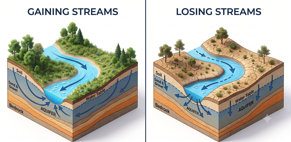
The hydraulic relationship between a river and an aquifer (the geological formation storing groundwater) is broadly classified into two categories based on the relative elevations of the water table and the river stage (Freeze and Cherry 1979).

Figure 1: Hydraulic relationship between a river and groundwater. When the water table is higher than the river stage, groundwater discharges into the river (gaining stream). When it is lower, river water infiltrates into the aquifer (losing stream).

When viewed from above as a “plan view,” the relationship between the river and groundwater flow becomes even clearer.

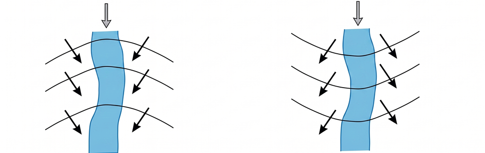
Figure 2: Plan view showing equipotential lines and flowlines for gaining (left) and losing (right) streams.

In the plan view (Figure 2), the curved black lines represent equipotential lines (groundwater contours), and the arrows indicate flowlines showing the direction of groundwater movement. Groundwater always flows perpendicular to the equipotential lines, from higher to lower hydraulic head. For a gaining stream (left), the contours form a “V” shape pointing upstream, with flow converging into the river. Conversely, for a losing stream (right), the contours form an inverted “V” shape, with flow diverging away from the river.

2.1 Gaining Stream

A gaining stream occurs when the surrounding water table is higher than the river water level (stage) (Figure 1 Left). Under these conditions, groundwater flows from the aquifer into the river driven by the hydraulic gradient. Consequently, the streamflow increases in the downstream direction. In humid regions like Japan, most rivers remain in this “gaining” state throughout the year, which is the primary reason why they do not dry up during dry spells.

2.2 Losing Stream

A losing stream occurs when the surrounding water table is lower than the river stage (Figure 1 Right). In this case, river water leaks through the riverbed into the aquifer, driven by gravity and the hydraulic gradient. This phenomenon is commonly observed in arid regions or areas where the water table has been drawn down due to excessive groundwater pumping. The flow of such rivers decreases downstream, and some may dry up entirely.

3 Python Hands-on: Hydrograph Baseflow Separation

The streamflow hydrograph measured at a gauging station is a combination of “quickflow” (direct runoff following rainfall events) and “baseflow” (slow discharge from groundwater).

Separating these two components is crucial for estimating groundwater recharge rates and predicting water availability during dry seasons. In this hands-on section, we will implement the Lyne-Hollick digital filter method, a classic technique in hydrology, using Python to separate baseflow from a synthetic hydrograph.

3.1 The Lyne-Hollick Filter Algorithm

The method proposed by Lyne & Hollick (Lyne and Hollick 1979) uses a digital low-pass filter, analogous to signal processing, to remove quickflow (high-frequency components) and isolate baseflow (low-frequency components).

\[ q_t = \alpha q_{t-1} + \frac{1+\alpha}{2} (Q_t - Q_{t-1}) \]

\[ b_t = Q_t - q_t \]

Where the variables are defined as: * \(Q_t\): total streamflow at time step \(t\) (\(m^3/s\)) * \(q_t\): quickflow at time step \(t\) (\(m^3/s\)) * \(b_t\): baseflow at time step \(t\) (\(m^3/s\)) * \(\alpha\): filter parameter (typically ranges from 0.90 to 0.995; a larger value yields a smoother baseflow. A value of 0.925 is commonly used for daily flow data)

Note: The constraints \(q_t \ge 0\) and \(b_t \ge 0\) (implying \(q_t \le Q_t\)) must be satisfied at each step. To eliminate phase shift, it is standard practice to run the filter forward, reverse the time series and run it backward, and then average the results (Forward-Backward pass) (Chapman 1991).

3.2 Implementation Code

The following script generates a synthetic hydrograph with storm peaks, applies the digital filter, and plots the results (this is the exact script used to generate the figure in this post).

import numpy as np
import matplotlib.pyplot as plt

# 1. Generate synthetic hydrograph data
np.random.seed(42)
days = 90
t = np.arange(days)

# Smooth baseflow representing groundwater contribution (true curve)
baseflow_true = 15.0 * np.exp(-t / 120.0) + 5.0 * np.sin(2.0 * np.pi * t / 365.0) + 10.0

# Storm-induced quickflow
quickflow = np.zeros(days)
storm_days = [15, 45, 70]
storm_magnitudes = [45.0, 60.0, 35.0]

for sd, mag in zip(storm_days, storm_magnitudes):
    for i in range(days):
        if i >= sd:
            quickflow[i] += mag * np.exp(-(i - sd) / 3.0)  # Exponential recession

# Total streamflow = baseflow + quickflow + noise
total_flow = baseflow_true + quickflow + np.random.normal(0, 0.5, days)
total_flow = np.clip(total_flow, 1.0, None)

# 2. Apply the Lyne-Hollick Digital Filter (Forward-Backward Pass)
alpha = 0.925

# Forward Pass
q_f = np.zeros(days)
for i in range(1, days):
    q_f[i] = alpha * q_f[i-1] + 0.5 * (1 + alpha) * (total_flow[i] - total_flow[i-1])
    if q_f[i] < 0:
        q_f[i] = 0
    elif q_f[i] > total_flow[i]:
        q_f[i] = total_flow[i]

# Backward Pass
q_b = np.zeros(days)
for i in range(days-2, -1, -1):
    q_b[i] = alpha * q_b[i+1] + 0.5 * (1 + alpha) * (total_flow[i] - total_flow[i+1])
    if q_b[i] < 0:
        q_b[i] = 0
    elif q_b[i] > total_flow[i]:
        q_b[i] = total_flow[i]

# Average estimated quickflow and calculate baseflow
q_est = 0.5 * (q_f + q_b)
q_est = np.clip(q_est, 0, total_flow)
baseflow_est = total_flow - q_est

# 3. Create a premium plot
fig, ax = plt.subplots(figsize=(10, 6))
fig.patch.set_facecolor('#F8F9FA')
ax.set_facecolor('#F8F9FA')

ax.plot(t, total_flow, color='#1A365D', linewidth=2, label="Total Streamflow Q(t)", zorder=4)
ax.fill_between(t, 0, baseflow_est, color='#90E0EF', alpha=0.8, label="Estimated Baseflow (GW Discharge)", zorder=3)
ax.fill_between(t, baseflow_est, total_flow, color='#F6AD55', alpha=0.5, label="Estimated Quickflow (Runoff)", zorder=2)

ax.set_xlabel("Elapsed Days", fontsize=12, fontweight='bold', color='#2D3748')
ax.set_ylabel("Discharge (m³/s)", fontsize=12, fontweight='bold', color='#2D3748')
ax.set_title("Hydrograph Baseflow Separation", fontsize=16, fontweight='bold', color='#1A365D', pad=15)
ax.set_xlim(0, days-1)
ax.set_ylim(0, 100)
ax.spines['top'].set_visible(False)
ax.spines['right'].set_visible(False)
ax.spines['left'].set_color('#CBD5E0')
ax.spines['bottom'].set_color('#CBD5E0')
ax.grid(axis='y', alpha=0.4, color='#E2E8F0', linestyle='--')
ax.legend(loc="upper right", frameon=True, facecolor='#F8F9FA', edgecolor='#CBD5E0')

plt.tight_layout()
plt.show()

3.3 Code Explanation for Beginners

Let’s break down what the Python script above is actually doing, step-by-step.

np.random.seed(42) and Data Generation First, we create some dummy data for our experiment. baseflow_true represents the “slowly changing groundwater,” while quickflow represents the “sudden surge of water after rain.” Adding these together gives us the total_flow.
q_f = np.zeros(days) and the for Loop np.zeros creates an empty box (an array) filled with zeros. The for i in range(...) loop then goes through each day, adding a little bit of “yesterday’s flow” to “today’s flow change.” This step-by-step accumulation is the core of the digital filter.
Safety Net with np.clip To prevent physically impossible numbers—like calculating that “more groundwater is discharging than the total river flow”—we use the np.clip function. This strictly caps the calculated values so they stay between 0 and the actual total flow.
Forward-Backward Pass If we only calculate forward in time, the resulting graph gets slightly shifted to the right (a delay). To fix this, we calculate forward, then calculate backward from the future to the past, and average the two. This ensures the peak aligns perfectly with the rain event.

3.4 Analysis of the Filter Results

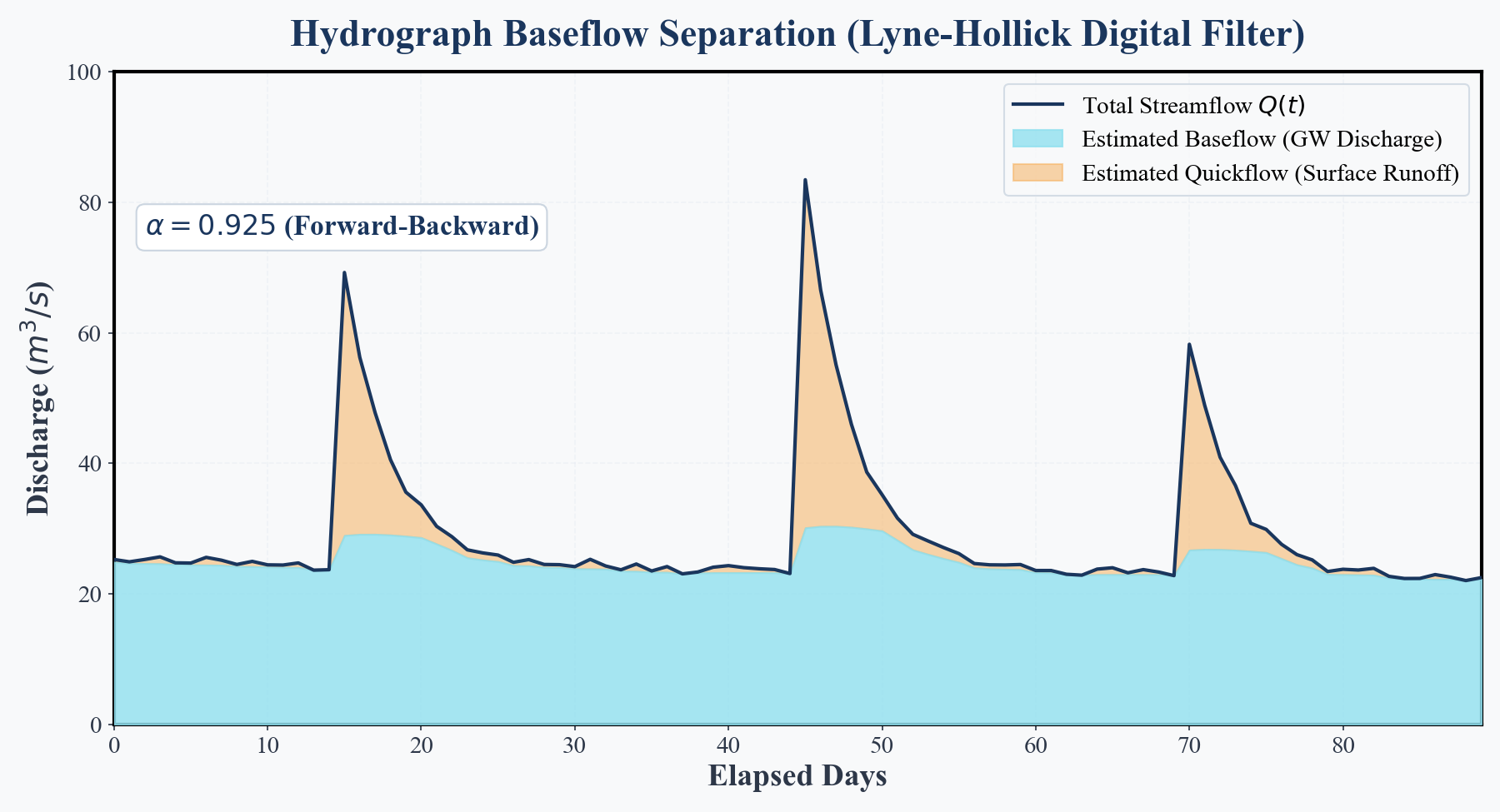
Figure 3: Baseflow separation results using the Lyne-Hollick digital filter. The sharp runoff peaks (orange) have been removed, leaving the smooth, delayed groundwater contribution (light blue).

The separation results (Figure 3) show that during storm events when the total flow spikes, the estimated baseflow (light blue region) does not rise abruptly. Instead, it reaches a delayed, muted peak and then recedes very slowly over time.

This gradual, sustained curve embodies the “memory” of the groundwater system, which acts as a massive natural reservoir filtering out the high-frequency variations of rainfall.

4 Conclusion: Conjunctive Management of Rivers and Groundwater

Let’s review the key concepts covered in this article:

Baseflow is the source of dry-weather river flow and is primarily supplied by groundwater discharge.
The connection between a river and an aquifer is defined by the head difference, classifying reach dynamics into gaining reaches (GW discharges to stream) and losing reaches (stream leaks to GW).
Using the Lyne-Hollick digital filter in Python, we can quantitatively partition a stream hydrograph into baseflow and quickflow.

To address river pollution or water scarcity, it is insufficient to manage surface water alone. We must view surface water and groundwater as a single, hydraulically connected resource, managing them conjunctively (conjunctive management) to achieve sustainable water use.

5 Next Episode Preview

In the next episode, we will focus on Groundwater Chemistry.

Why does groundwater taste and contain different constituents depending on where it is sampled? How does water react with minerals in the aquifer as it moves along flow paths? We will combine Python and PHREEQC to plot Piper diagrams and Stiff diagrams, learning how to decipher the “geochemical resume” of groundwater.

6 References

Chapman, Tom G. 1991. “Comment on "Evaluation of Automated Techniques for Estimating Trigger and Baseflow Fractions in Streamflow" by Nathan, r. J. And McMahon, t. a.” Water Resources Research 27 (7): 1783–84.

Freeze, R. Allan, and John A. Cherry. 1979. Groundwater. Prentice-Hall.

Lyne, Vincent, and Malcolm Hollick. 1979. “Forest Hydrology in Relation to Water Management.” National Conference on Institution of Engineers Australia (Canberra), 109–18.